An introduction to probabilistic programming, now available in TensorFlow Probability
十二月 10, 2018
Posted by Mike Shwe, Product Manager for TensorFlow Probability at Google; Josh Dillon, Software Engineer for TensorFlow Probability at Google; Bryan Seybold, Software Engineer at Google; Matthew McAteer; and Cam Davidson-Pilon.

New to probabilistic programming? New to TensorFlow Probability (TFP)? Then we’ve got something for you. Bayesian Methods for Hackers, an introductory, hands-on tutorial, is now available with examples in TFP. Available as an open-source resource for all, the TFP version complements the previous one written in PyMC3.

There’s a number of neat things about Bayesian Methods for Hackers: not only is it approachable for the probabilistic novice, but it also demonstrates how to apply probabilistic programming to real-world problems.

Probabilistic programming for everyone

Though not required for probabilistic programming, the Bayesian approach offers an intuitive framework for representing beliefs and updating those beliefs based on new data. Bayesian Methods for Hackers teaches these techniques in a hands-on way, using TFP as a substrate. Since the book is written in Google Colab, you’re invited to run and modify the Python examples.

The TensorFlow team built TFP for data scientists, statisticians, and ML researchers and practitioners who want to encode domain knowledge to understand data and make predictions. TFP is a Python library built on TensorFlow that makes it easy to combine probabilistic models and deep learning on modern hardware. TFP allows you to:

  • Explore your data interactively
  • Evaluate different models rapidly
  • Leverage modern, vectorized hardware accelerators automatically
  • Launch easily and with confidence. TFP is professionally built and tested, Google-Cloud ready, and supported by a vibrant open source community.

As we discuss in related blog posts, probabilistic programming has diverse applications, including finance and the oil and gas industry. Why? Uncertainty is ubiquitous. Real-world phenomena — even those we completely understand — are subject to externalities beyond our control or even awareness. Dismissing these factors means conclusions might be wrong or at best misleading. We’ve built TFP to be accessible to all, to model the uncertainty all around us.

Addressing real-world problems

Many Bayesian tutorials focus on working through easy problems which have analytical solutions: think coin flips and dice rolls. While Bayesian Methods for Hackers starts with these, it quickly moves onto more realistic problems. Examples range from understanding the cosmos to detecting a change in an online user’s behavior.

In the remainder of this blog, we’ll provide an overview of a famous real-world problem that gets more detailed treatment in the Bayesian Hackers book in Chapter 2: the 1986 Space Shuttle Challenger disaster.

On January 28, 1986 on the 25th flight of the U.S. Space Shuttle, one of the two solid rocket boosters on the Shuttle Challenger exploded, due to an O-ring failure. Although mission engineers had numerous communications with the manufacturer of the O-ring about damage on previous flights, the manufacturer deemed the risk to be acceptable [1].

Below, we depict the observations of seven O-ring damage incidents on prior shuttle missions, as a function of ambient temperature. (At 70 degrees, there are two incidents.)
graph showing observations of seven O-ring damage incidents on prior shuttle missions, as a function of ambient temperature.
You’ll note that as the temperature decreases, there’s clearly an increase in proportion of damaged O-rings, yet there’s not an obvious temperature threshold below which the O-rings would likely fail. As with most real-world phenomena, there is uncertainty involved. We wish to determine at a given temperature t, what is the probability of an O-ring failure?

We can model the probability p of O-ring damage at temperature t using a logistic function, in particular:
log function
where β determines the shape of the logistic function and 𝛼 is the bias term, shifting the function from left to right. Since both of these parameters can be positive or negative with no particular bounds or biases in size, we can model them as gaussian random variables:
log function
In TFP, we can intuitively represent 𝛼 and β with tfp.distributions.Normal, as in this code snippet:
temperature_ = challenger_data_[:, 0]
temperature = tf.convert_to_tensor(temperature_, dtype=tf.float32)
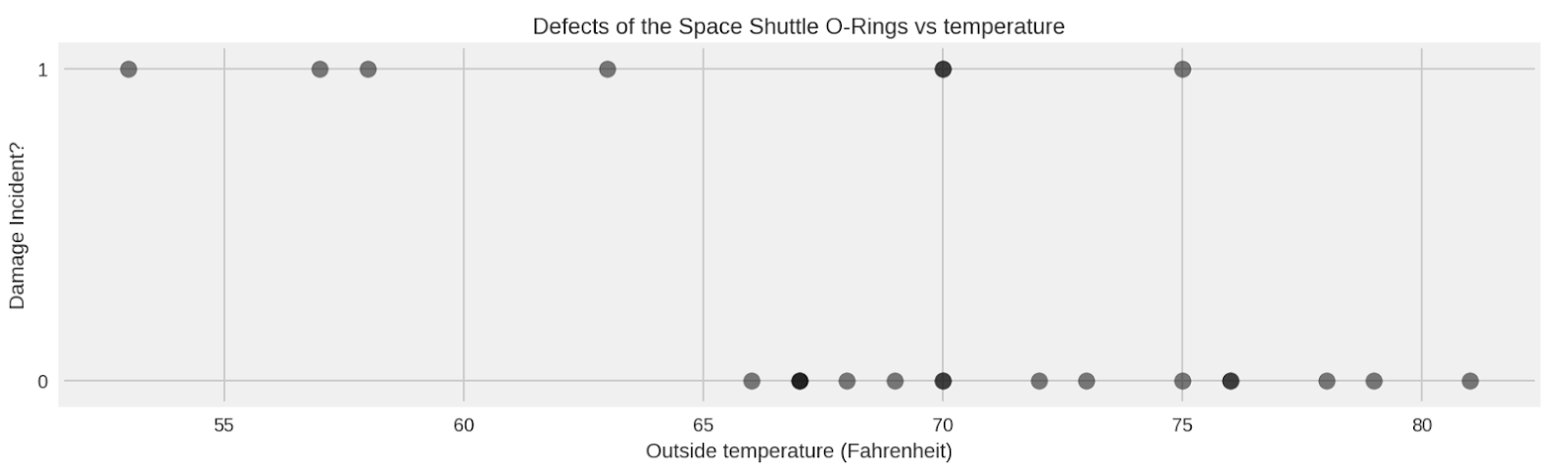
D_ = challenger_data_[:, 1]                # defect or not?
D = tf.convert_to_tensor(D_, dtype=tf.float32)

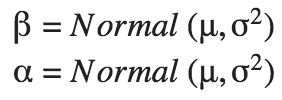
beta = tfd.Normal(name="beta", loc=0.3, scale=1000.).sample()
alpha = tfd.Normal(name="alpha", loc=-15., scale=1000.).sample()
p_deterministic = tfd.Deterministic(name="p", loc=1.0/(1. + tf.exp(beta * temperature_ + alpha))).sample()

[
    prior_alpha_,
    prior_beta_,
    p_deterministic_,
    D_,
] = evaluate([
    alpha,
    beta,
    p_deterministic,
    D,
])
(To run this code snippet, head on over to the Google Colab version of Chapter 2, so you can run the entire Space Shuttle example).

Note that we get our actual value of 0 or 1 for p(t) in line 8, wherein we’re sampling from the logistic function using the previously sampled values of 𝛼 and β in lines 6 and 7. Also, note that the evaluate() helper function allows us to transition between graph and eager modes seamlessly, while converting tensor values to numpy. We describe eager and graph modes, as well as this helper function in more detail in the beginning of Chapter 2.

To connect the probability of failure at temperature t, p(t), to our observed data we can use a Bernoulli random variable with parameter p(t). Note that in general, Ber(p) is a random variable that takes value 1 with probability p, and 0 otherwise. So, the last part of our generative model is that we have a defect incident D𝑖 at temperature value 𝑖 that can be modeled as:
Given this generative model, we want to find model parameters so that the model can explain our observed data — that’s the goal of probabilistic inference!

TFP performs probabilistic inference by evaluating the model using an unnormalized joint log probability function. The arguments to this joint_log_prob are data and model state. The function returns the log of the joint probability that the parameterized model generated the observed data. To learn more about the joint_log_prob, please see this vignette.

For the sake of the Challenger example, here’s how we define the joint_log_prob:
def challenger_joint_log_prob(D, temperature_, alpha, beta):
    """
    Joint log probability optimization function.
        
    Args:
      D: The Data from the challenger disaster representing presence or 
         absence of defect
      temperature_: The Data from the challenger disaster, specifically the temperature on 
         the days of the observation of the presence or absence of a defect
      alpha: one of the inputs of the HMC
      beta: one of the inputs of the HMC
    Returns: 
      Joint log probability optimization function.
    """
    rv_alpha = tfd.Normal(loc=0., scale=1000.)
    rv_beta = tfd.Normal(loc=0., scale=1000.)
    logistic_p = 1.0/(1. + tf.exp(beta * tf.to_float(temperature_) + alpha))
    rv_observed = tfd.Bernoulli(probs=logistic_p)
  
    return (
        rv_alpha.log_prob(alpha)
        + rv_beta.log_prob(beta)
        + tf.reduce_sum(rv_observed.log_prob(D))
    )
Notice how lines 15–18 succinctly encode our generative model, one line per random variable. Also, note that rv_alpha and rv_beta represent the random variables for our prior distributions for 𝛼 and β. By contrast, rv_observedrepresents the conditional distribution for the likelihood of observations in temperature and O-ring outcome, given a logistic distribution parameterized by 𝛼 and β.

Next, we take our joint_log_prob function, and send it to the tfp.mcmc module. Markov chain Monte Carlo (MCMC) algorithms make educated guesses about the unknown input values, computing the likelihood of the set of arguments in the joint_log_prob function. By repeating this process many times, MCMC builds a distribution of likely parameters. Constructing this distribution is the goal of probabilistic inference.

Accordingly, we’ll set up a particular type of MCMC, called Hamiltonian Monte Carlo, over our challenge_joint_log_prob function:
number_of_steps = 10000
burnin = 2000

# Set the chain's start state.
initial_chain_state = [
    0. * tf.ones([], dtype=tf.float32, name="init_alpha"),
    0. * tf.ones([], dtype=tf.float32, name="init_beta")
]

# Since HMC operates over unconstrained space, we need to transform the
# samples so they live in real-space.
# Alpha is 100x of beta approximately, so apply Affine scalar bijector
# to multiply the unconstrained alpha by 100 to get back to 
# the Challenger problem space
unconstraining_bijectors = [
    tfp.bijectors.AffineScalar(100.),
    tfp.bijectors.Identity()
]

# Define a closure over our joint_log_prob.
unnormalized_posterior_log_prob = lambda *args: challenger_joint_log_prob(D, temperature_, *args)

# Initialize the step_size. (It will be automatically adapted.)
with tf.variable_scope(tf.get_variable_scope(), reuse=tf.AUTO_REUSE):
    step_size = tf.get_variable(
        name='step_size',
        initializer=tf.constant(0.5, dtype=tf.float32),
        trainable=False,
        use_resource=True
    )

# Defining the HMC
hmc=tfp.mcmc.TransformedTransitionKernel(
    inner_kernel=tfp.mcmc.HamiltonianMonteCarlo(
        target_log_prob_fn=unnormalized_posterior_log_prob,
        num_leapfrog_steps=40, #to improve convergence
        step_size=step_size,
        step_size_update_fn=tfp.mcmc.make_simple_step_size_update_policy(
            num_adaptation_steps=int(burnin * 0.8)),
        state_gradients_are_stopped=True),
    bijector=unconstraining_bijectors)

# Sampling from the chain.
[
    posterior_alpha,
    posterior_beta
], kernel_results = tfp.mcmc.sample_chain(
    num_results = number_of_steps,
    num_burnin_steps = burnin,
    current_state=initial_chain_state,
    kernel=hmc)

# Initialize any created variables for preconditions
init_g = tf.global_variables_initializer()
Finally, we’ll actually perform the inference, through our evaluate() helper function:
evaluate(init_g)
[
    posterior_alpha_,
    posterior_beta_,
    kernel_results_
] = evaluate([
    posterior_alpha,
    posterior_beta,
    kernel_results
])
    
print("acceptance rate: {}".format(
    kernel_results_.inner_results.is_accepted.mean()))
print("final step size: {}".format(
    kernel_results_.inner_results.extra.step_size_assign[-100:].mean()))
Plotting the distributions for 𝛼 and β, we note that the distributions are fairly wide, as one would expect with so few data points and overlap in temperature between failure and non-failure observations. Yet, even with the wide distributions, we can be fairly confident that temperature does indeed have an effect on the probability of O-ring damage, since all of the samples of β are greater than 0. We can likewise be confident that α is significantly less than 0, since all samples are well into the negative.
Graph Plotting the distributions for 𝛼 and β
As we mentioned above, what we really want to know is: What is the expected probability of O-ring damage at a given temperature? To compute this probability, we can average over all samples from the posterior to get a likely value for p(t𝑖).
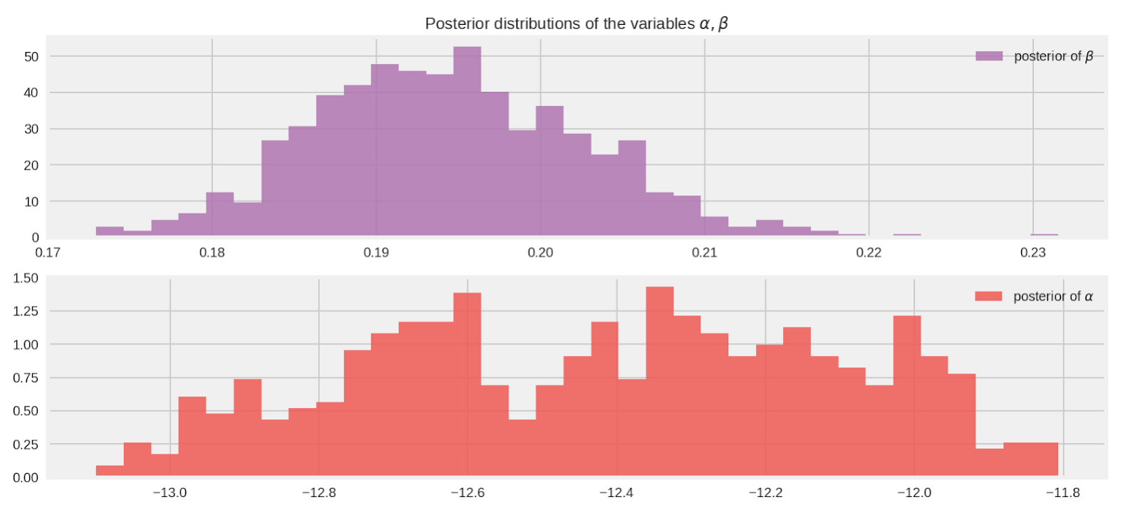
alpha_samples_1d_ = posterior_alpha_[:, None]  # best to make them 1d
beta_samples_1d_ = posterior_beta_[:, None]

beta_mean = tf.reduce_mean(beta_samples_1d_.T[0])
alpha_mean = tf.reduce_mean(alpha_samples_1d_.T[0])
[ beta_mean_, alpha_mean_ ] = evaluate([ beta_mean, alpha_mean ])

print("beta mean:", beta_mean_)
print("alpha mean:", alpha_mean_)
def logistic(x, beta, alpha=0):
    """
    Logistic function with alpha and beta.
        
    Args:
      x: independent variable
      beta: beta term 
      alpha: alpha term
    Returns: 
      Logistic function
    """
    return 1.0 / (1.0 + tf.exp((beta * x) + alpha))

t_ = np.linspace(temperature_.min() - 5, temperature_.max() + 5, 2500)[:, None]
p_t = logistic(t_.T, beta_samples_1d_, alpha_samples_1d_)
mean_prob_t = logistic(t_.T, beta_mean_, alpha_mean_)
[ 
    p_t_, mean_prob_t_
] = evaluate([ 
    p_t, mean_prob_t
])
We can then compute a 95% credible interval across the range of temperatures. Note that this is a credible interval, not a confidence interval typically found in frequentist approaches to statistical analysis. The 95% credible intervals tells us that we can be 95% sure that the true value will lie within the interval. For example, as we depict below with the purple region, at 50 degrees, we can be 95% sure that the probability of failure lies between 1.0 and 0.80. Ironically, many people erroneously interpret a confidence interval to have this property.

On the day of the Challenger disaster, at 31 degrees, it turns out that the posterior distribution for an O-ring failure would lead us to conclude with a high degree of confidence that a problem would occur.

This rather straightforward probabilistic analysis demonstrates the power of TFP and Bayesian methods: that they can be used to provide valuable insight and prediction into real-world problems of significant consequence.

Read on!

You’ll find a cornucopia of real-world examples in the Bayesian Hackers book. An analysis of text-messaging volume over time that you can apply to a wide variety of fault detection problems in manufacturing and production systems. Software engineers at Google applied the methods for the text-messaging analysis to understanding text flakiness for production software — within a few weeks after we first drafted the TFP version of the chapter.

You’ll also find an analysis to find dark matter in the universe. Also, predicting returns of shares in public companies, i.e., stock returns.

We hope that you’ll dig into the conceptual walkthroughs in the book, applying the techniques to problems in your field. Please help us to keep this book in top shape by making comments and pull requests in the github!

Acknowledgements

We thank the TensorFlow Probability team for their assistance in writing the TFP version of the Bayesian Hackers book.

References

[1] https://en.wikipedia.org/wiki/Space_Shuttle_Challenger_disaster
Next post
An introduction to probabilistic programming, now available in TensorFlow Probability

Posted by Mike Shwe, Product Manager for TensorFlow Probability at Google; Josh Dillon, Software Engineer for TensorFlow Probability at Google; Bryan Seybold, Software Engineer at Google; Matthew McAteer; and Cam Davidson-Pilon.

New to probabilistic programming? New to TensorFlow Probability (TFP)? Then we’ve got something for you. Bayesian Methods for Hackers, an introductory, hands-on tutorial,…