This article is also shared on the Google Research Blog

Objects and their relationships are ubiquitous in the world around us, and relationships can be as important to understanding an object as its own attributes viewed in isolation — for example: transportation networks, production networks, knowledge graphs, or social networks. Discrete mathematics and computer science have a long history of formalizing such networks them as graphs, consisting of nodes arbitrarily connected by edges in various irregular ways. Yet most machine learning (ML) algorithms allow only for regular and uniform relations between input objects, such as a grid of pixels, a sequence of words, or no relation at all.

Graph neural networks, or GNNs for short, have emerged as a powerful technique to leverage both the graph’s connectivity (as in the older algorithms DeepWalk and Node2Vec) and the input features on the various nodes and edges. GNNs can make predictions for graphs as a whole (Does this molecule react in a certain way?), for individual nodes (What’s the topic of this document, given its citations?) or for potential edges (Is this product likely to be purchased together with that product?). Apart from making predictions about graphs, GNNs are a powerful tool used to bridge the chasm to more typical neural network use cases. They encode a graph's discrete, relational information in a continuous way so that it can be included naturally in another deep learning system.

We are excited to announce the release of TensorFlow GNN 1.0 (TF-GNN), a production-tested library for building GNNs at large scale. It supports both modeling and training in TensorFlow as well as the extraction of input graphs from huge data stores. TF-GNN is built from the ground up for heterogeneous graphs where types and relations are represented by distinct sets of nodes and edges. Real-world objects and their relations occur in distinct types and TF-GNN's heterogeneous focus makes it natural to represent them.

Inside TensorFlow, such graphs are represented by objects of type tfgnn.GraphTensor. This is a composite tensor type (a collection of tensors in one Python class) accepted as a first-class citizen in tf.data.Dataset, tf.function, etc. It stores both the graph structure and its features attached to nodes, edges and the graph as a whole. Trainable transformations of GraphTensors can be defined as Layers objects in the high-level Keras API, or directly using the tfgnn.GraphTensor primitive.

GNNs: Making predictions for an object in context

For illustration, let’s look at one typical application of TF-GNN: predicting a property of a certain type of node in a graph defined by cross-referencing tables of a huge database. For example, a citation database of Computer Science (CS) arXiv papers with one-to-many cites and many-to-one cited relationships where we would like to predict the subject area of each paper.

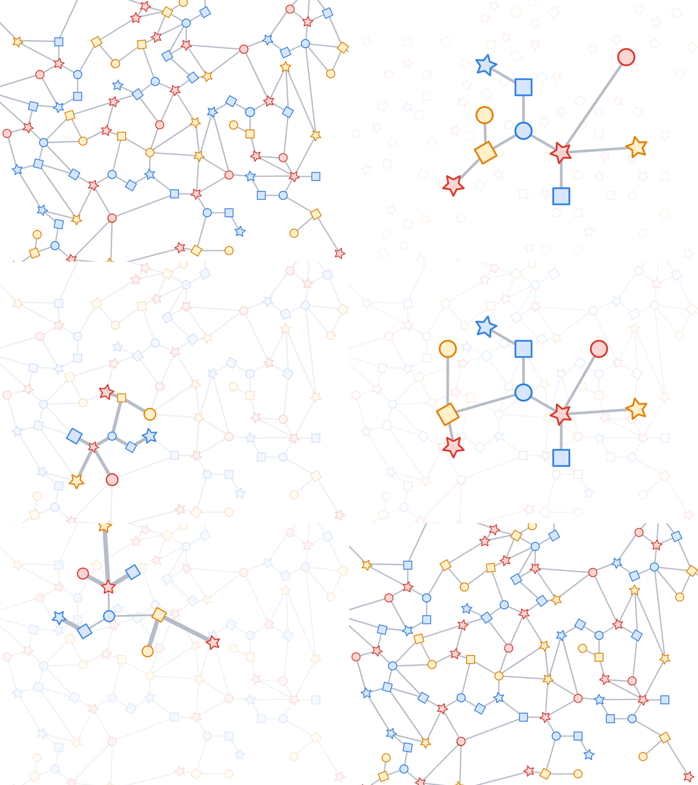
Like most neural networks, a GNN is trained on a dataset of many labeled examples (~millions), but each training step consists only of a much smaller batch of training examples (say, hundreds). To scale to millions, the GNN gets trained on a stream of reasonably small subgraphs from the underlying graph. Each subgraph contains enough of the original data to compute the GNN result for the labeled node at its center and train the model. This process — typically referred to as subgraph sampling — is extremely consequential for GNN training. Most existing tooling accomplishes sampling in a batch way, producing static subgraphs for training. TF-GNN provides tooling to improve on this by sampling dynamically and interactively.

Pictured, the process of subgraph sampling where small, tractable subgraphs are sampled from a larger graph to create input examples for GNN training.

TF-GNN 1.0 debuts a flexible Python API to configure dynamic or batch subgraph sampling at all relevant scales: interactively in a Colab notebook (like this one), for efficient sampling of a small dataset stored in the main memory of a single training host, or distributed by Apache Beam for huge datasets stored on a network filesystem (up to hundreds of millions of nodes and billions of edges). For details, please refer to our user guides for in-memory and beam-based sampling, respectively.

On those same sampled subgraphs, the GNN’s task is to compute a hidden (or latent) state at the root node; the hidden state aggregates and encodes the relevant information of the root node's neighborhood. One classical approach is message-passing neural networks. In each round of message passing, nodes receive messages from their neighbors along incoming edges and update their own hidden state from them. After n rounds, the hidden state of the root node reflects the aggregate information from all nodes within n edges (pictured below for n = 2). The messages and the new hidden states are computed by hidden layers of the neural network. In a heterogeneous graph, it often makes sense to use separately trained hidden layers for the different types of nodes and edges.

Pictured, a simple message-passing neural network where, at each step, the node state is propagated from outer to inner nodes where it is pooled to compute new node states. Once the root node is reached, a final prediction can be made.

The training setup is completed by placing an output layer on top of the GNN’s hidden state for the labeled nodes, computing the loss (to measure the prediction error), and updating model weights by backpropagation, as usual in any neural network training.

Beyond supervised training (i.e., minimizing a loss defined by labels), GNNs can also be trained in an unsupervised way (i.e., without labels). This lets us compute a continuous representation (or embedding) of the discrete graph structure of nodes and their features. These representations are then typically utilized in other ML systems. In this way, the discrete, relational information encoded by a graph can be included in more typical neural network use cases. TF-GNN supports a fine-grained specification of unsupervised objectives for heterogeneous graphs.

Building GNN architectures

The TF-GNN library supports building and training GNNs at various levels of abstraction.

At the highest level, users can take any of the predefined models bundled with the library that are expressed in Keras layers. Besides a small collection of models from the research literature, TF-GNN comes with a highly configurable model template that provides a curated selection of modeling choices that we have found to provide strong baselines on many of our in-house problems. The templates implement GNN layers; users need only to initialize the Keras layers.

import tensorflow_gnn as tfgnn
from tensorflow_gnn.models import mt_albis

def model_fn(graph_tensor_spec: tfgnn.GraphTensorSpec):
  """Builds a GNN as a Keras model."""
  graph = inputs = tf.keras.Input(type_spec=graph_tensor_spec)

  # Encode input features (callback omitted for brevity).
  graph = tfgnn.keras.layers.MapFeatures(
      node_sets_fn=set_initial_node_states)(graph)

  # For each round of message passing...
  for _ in range(2):
    # ... create and apply a Keras layer.
    graph = mt_albis.MtAlbisGraphUpdate(
        units=128, message_dim=64,
        attention_type="none", simple_conv_reduce_type="mean",
        normalization_type="layer", next_state_type="residual",
        state_dropout_rate=0.2, l2_regularization=1e-5,
    )(graph)

  return tf.keras.Model(inputs, graph)

At the lowest level, users can write a GNN model from scratch in terms of primitives for passing data around the graph, such as broadcasting data from a node to all its outgoing edges or pooling data into a node from all its incoming edges (e.g., computing the sum of incoming messages). TF-GNN’s graph data model treats nodes, edges and whole input graphs equally when it comes to features or hidden states, making it straightforward to express not only node-centric models like the MPNN discussed above but also more general forms of GraphNets. This can, but need not, be done with Keras as a modeling framework on the top of core TensorFlow. For more details, and intermediate levels of modeling, see the TF-GNN user guide and model collection.

Training orchestration

While advanced users are free to do custom model training, the TF-GNN Runner also provides a succinct way to orchestrate the training of Keras models in the common cases. A simple invocation may look like this:

from tensorflow_gnn import runner

runner.run(
   task=runner.RootNodeBinaryClassification("papers", ...),
   model_fn=model_fn,
   trainer=runner.KerasTrainer(tf.distribute.MirroredStrategy(), model_dir="/tmp/model"),
   optimizer_fn=tf.keras.optimizers.Adam,
   epochs=10,
   global_batch_size=128,
   train_ds_provider=runner.TFRecordDatasetProvider("/tmp/train*"),
   valid_ds_provider=runner.TFRecordDatasetProvider("/tmp/validation*"),
   gtspec=...,
)

The Runner provides ready-to-use solutions for ML pains like distributed training and tfgnn.GraphTensor padding for fixed shapes on Cloud TPUs. Beyond training on a single task (as shown above), it supports joint training on multiple (two or more) tasks in concert. For example, unsupervised tasks can be mixed with supervised ones to inform a final continuous representation (or embedding) with application specific inductive biases. Callers only need substitute the task argument with a mapping of tasks:

from tensorflow_gnn import runner
from tensorflow_gnn.models import contrastive_losses

runner.run(
     task={
        "classification": runner.RootNodeBinaryClassification("papers", ...),
        "dgi": contrastive_losses.DeepGraphInfomaxTask("papers"),
      },
    ...
)

Additionally, the TF-GNN Runner also includes an implementation of integrated gradients for use in model attribution. Integrated gradients output is a GraphTensor with the same connectivity as the observed GraphTensor but its features replaced with gradient values where larger values contribute more than smaller values in the GNN prediction. Users can inspect gradient values to see which features their GNN uses the most.

Conclusion

In short, we hope TF-GNN will be useful to advance the application of GNNs in TensorFlow at scale and fuel further innovation in the field. If you’re curious to find out more, please try our Colab demo with the popular OGBN-MAG benchmark (in your browser, no installation required), browse the rest of our user guides and Colabs, or take a look at our paper.

Acknowledgements

The TF-GNN release 1.0 was developed by a collaboration between Google Research (Sami Abu-El-Haija, Neslihan Bulut, Bahar Fatemi, Johannes Gasteiger, Pedro Gonnet, Jonathan Halcrow, Liangze Jiang, Silvio Lattanzi, Brandon Mayer, Vahab Mirrokni, Bryan Perozzi, Anton Tsitsulin, Dustin Zelle), Google Core ML (Arno Eigenwillig, Oleksandr Ferludin, Parth Kothari, Mihir Paradkar, Jan Pfeifer, Rachael Tamakloe), and Google DeepMind (Alvaro Sanchez-Gonzalez and Lisa Wang).