MIT 6.S191: Introduction to Deep Learning is an introductory course offered formally offered at MIT and open-sourced on the course website. The class consists of a series of foundational lectures on the fundamentals of neural networks, its applications to sequence modeling, computer vision, generative models, and reinforcement learning.MIT 6.S…
MIT 6.S191: Introduction to Deep Learning is an introductory course offered formally offered at MIT and open-sourced on the course website. The class consists of a series of foundational lectures on the fundamentals of neural networks, its applications to sequence modeling, computer vision, generative models, and reinforcement learning.
MIT 6.S191: MIT’s official introductory course on deep learning algorithms and their applications
MIT 6.S191 is more than just another lecture series on deep learning. In designing the course, we wanted to do something more. We wanted to equip our audience with the practical skills necessary to go out and implement their own deep learning models, to apply what they got out of this course to the questions that excite and inspire them.
And so, we turned to TensorFlow. We designed two TensorFlow based software labs, focusing on music generation with recurrent neural networks and pneumothorax detection in medical images, to complement the course lectures. The TensorFlow labs gave students an opportunity to apply the fundamentals to two interesting, relevant problems and to build and refine their TensorFlow skills.
The material in 6.S191 is designed to be as accessible as possible, for people from varying backgrounds and levels of experience and for both the MIT community and beyond.
Accordingly, the first lab takes students through TensorFlow basics — building and executing computation graphs, sessions, and common operations used in deep learning. This introduction also highlights some of the latest and greatest that TensorFlow has to offer: the imperative version of TensorFlow, Eager mode.
This background sets students up to build models in TensorFlow for music generation and for pneumothorax detection in chest x-rays.
. . .
Music Generation with Recurrent Neural Networks
Recurrent neural networks (RNNs) are extensively used in sequence modeling and prediction tasks, on everything from stock trends, to natural language processing, to medical signals like EKGs. Check out our course lecture on deep sequence modeling for some background on RNNs and their applications.
RNNs are well suited for music generation, as they can capture temporal dependencies in time-series data like music. In this first lab, students work through encoding a dataset of music files, defining a RNN model in TensorFlow, and sampling from the model to generate new music that has never been heard before.
RNN Model for Music Generation
The dataset is a set of pop song snippets that are encoded into vector format to feed into the RNN model. Once the data is processed, the next step is to define and train a RNN model using this dataset of pop song snippets.
The model is based off a single long short-term memory (LSTM) cell, where the state vector tracks the temporal dependencies between consecutive notes. At each time step, a sequence of previous notes is fed into the cell, and the final output of the last unit in our LSTM is fed into a fully connected layer. Thus, we can output a probability distribution over the next note at time step t given the notes at all previous time steps. We visualize this process in the diagram below:
Predicting the likelihood of the next musical note in a sequence
We provided students with a guide to building the RNN model and defining the appropriate computation graph. Again, we’ve designed these labs to be accessible to everyone who’s interested, regardless of their prior experience with TensorFlow, so they’re guided for a reason!
The lab first goes through setting the relevant hyperparameters, defining placeholder variables, and initializing the weights for the RNN model. Students then worked to define their own function RNN(input_vec, weights, biases) that takes in the corresponding input variables and defines a computation graph.
The lab allows students to experiment with various loss functions, optimization schemes, and even accuracy metrics:
The fun doesn’t end with building and training an RNN! After all, this lab is about music generation — what’s left is to use this RNN to actually create new music.
The lab guides students through feeding the trained model a seed (after all, it can’t predict any new notes without something to start with!), and then iteratively predicting each successive note using the trained RNN. This amounts to randomly sampling from the probability distribution over the next note that’s outputted by the RNN at each time step, and then using these samples to generate a new song.
As before, we gave students a guided structure for doing this, but defining the sampling was all on them.
To provide a sampling (pun intended) of generated songs, we went ahead and trained a model, then sampled from it to generate new songs. Listen in on an example generated with a trained model:
Producing More Realistic Music
As one can probably tell, there’s a lot of room for improvement here. We wanted students to play around with the skeleton we provided, by tuning hyperparameters, placing priors over the distributions, and augmenting the dataset to generate even sweeter sounding music.
. . .
Pneumothorax Detection from Human X-Ray Scans
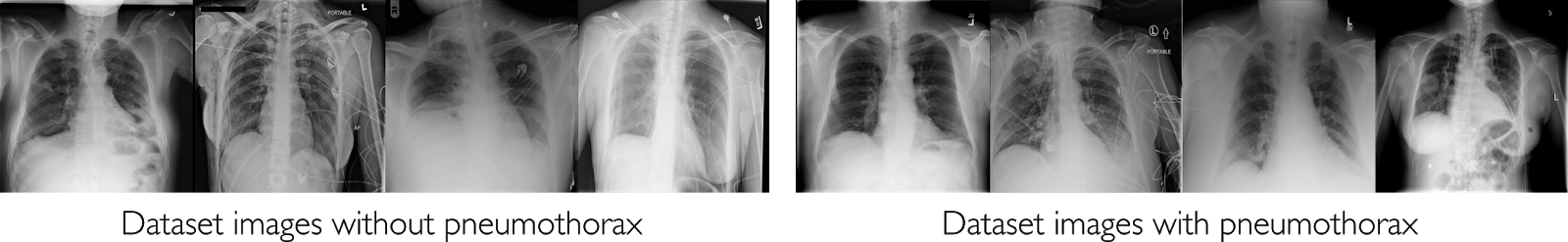
Our second lab complements a lecture on deep learning for computer vision. Students had the opportunity to use convolutional neural networks (CNNs) for disease detection on a realistic medical image dataset. Specifically, students used a set of real chest x-rays to build a model to detect and classify scans predicted to have pneumothorax, a condition that occurs when there is an abnormal amount of air in the space between the lung and the chest wall.
We took this lab a step beyond classification to try to address the notion of explainability — what are quantitative metrics that reflect why and how the network assigned a particular class label to a given image? To address this question, students implemented a technique for feature visualization called class activation mapping to gain an understanding of discriminative image regions.
Dataset
We utilized a subset of the ChestXRay dataset, which, as the name suggests, is a large dataset of chest x-rays labelled with corresponding diagnoses.
Since this is a real dataset, it is quite noisy. We wanted to have students work with real data so that they could get a sense of some of the challenges in curating and annotating data, particularly in the context of computer vision.
The CNN Model
Students worked with a pre-trained CNN for the pneumothorax detection task; rather than hiding this away in a black box, we provide the code for both the model as well as the call to train the model, and expected students to go through this as part of the lab. Additionally, the lab goes through implementing cost and prediction functions as well as evaluation metrics (such as ROC curves) for the CNN classifier.
CNN architecture for pneumothorax detection
Interpreting the CNN Output with CAMs
The main focus of this lab was on implementing class activation maps (CAMs) and using them to interpret the CNN’s output. While there are a lot of resources out there for CNN models for image classification, we found that there were few guided introductions or labs that also addressed the notion of interpretability. It’s important for us to help students recognize and appreciate some of the limitations of deep learning, both as part of this lab and as part of the course more generally. Incorporating CAMs into the lab also serves as an opportunity for students to read through and actually implement results from recent state of the art research — which (we think) is pretty awesome.
To provide some background, CAM is a method to visualize the regions of an image that a CNN “attends” to in its last convolutional layer. Note that CAM visualization pertains to architectures with a global average pooling layer before the final fully connected layer, where we output the spatial average of the feature map of each unit at the last convolutional layer.
CAMs effectively highlight the parts of the input image that mattered the most in assigning a particular class label. Intuitively, the CAM for a class is based on each feature map’s importance in assigning an image to that class. Feature maps in CNNs reflect the presence of specific visual patterns (i.e. features) in the image. We compute the CAM by taking a sum of the feature maps weighted by the importance of that feature map. Thus, regions of the input image with large activations in important channels are given greater weight in a CAM, and thus appear “hotter”.
In the context of our pneumothorax classifier, this amounts to highlighting the pixels in a x-ray that were most important in detecting (or not detecting) pneumothorax.
Class Activation Mapping on the final feature maps
To make this concrete, let F_k represent the k-th feature map in the last convolutional layer of our CNN, and let w_k represent the weights between the k-th feature map and the fully connected layer. The class activation map for assigning pneumothorax is then given by:
After upsampling the resulting class activation map, we can visualize the regions of the chest x-ray most relevant to pneumothorax detection (at least from the network’s perspective).
The lab goes through the process of computing and visualizing CAMs in Tensorflow from start to finish. Students have to define a function for extracting the feature maps and weights for the CAM computation:
Students feed the extracted feature_maps from the last convolutional layer and dense_weights from the fully connected layer into a function for computing the CAM, and then define the upsampling procedure.
Class activation map for chest x-ray positive for pneumothorax
The CAM can finally be visualized as a heatmap over the input image, as shown in this example of a pneumothorax-positive chest x-ray.
Perhaps the best part of this lab was the discussions it spawned. Students were left to mull over instances in which the model incorrectly classified the input x-ray, what the CAM looked like in those instances, and what changes could be made to the model to address these limitations. Building algorithms to “look” inside the brain of the neural networks piqued students’ curiosity and gave them a taste of the importance of interpretability in machine learning.
. . .
These labs are unique to MIT 6.S191 and designed specifically for this course by the course staff. If you’re interested in participating in and engaging with MIT 6.S191, you can follow us on Twitter @mitdeeplearning, watch our lecture videos, and take a look at our labs. Huge thanks to our wonderful sponsors, our amazing course staff, and the Google team for making this class and blog possible!
Watch all of the MIT 6.S191 lectures online for free!
MIT 6.S191: Introduction to Deep Learning is an introductory course offered formally offered at MIT and open-sourced on the course website. The class consists of a series of foundational lectures on the fundamentals of neural networks, its applications to sequence modeling, computer vision, generative models, and reinforcement learning.MIT 6.S…