https://blog.tensorflow.org/2018/09/the-trinity-of-errors-in-financial-models.html?hl=es
https://blogger.googleusercontent.com/img/b/R29vZ2xl/AVvXsEh4rDvmcSesUu3yakNotDOAtIzrbgsDCJkoTuH7IngQAl9auAL1SGO6KTREkKt8bE8_zcDB3FxAfRUTOpaQXNiuG6lzqoDPc98W5_UAp4w7XoLT6uLtfkhBNmteOqzTQHPnjvY389mE5z4/s1600/diagram.png
The Trinity Of Errors In Financial Models: An Introductory Analysis Using TensorFlow Probability
By Deepak Kanungo, Founder and CEO of Hedged Capital LLC.
At
Hedged Capital, an AI-first financial trading and advisory firm, we use probabilistic models to trade the financial markets. In this first blog post, we explore three types of errors inherent in all financial models, with a simple example of a model in
Tensorflow Probability (TFP).
Finance Is Not Physics
Adam Smith, generally recognized as the founder of modern economics, was in awe of Newton’s laws of mechanics and gravitation [1]. Ever since then, economists have endeavored to make their discipline into a science like physics. They aspire to formulate theories that accurately explain and predict the economic activities of human beings at the micro and macro levels. This desire gathered momentum in the early 20th century with economists like Irving Fisher and culminated in the Econophysics movement of the late 20th century.

Despite all the complicated mathematics of modern finance, its theories are woefully inadequate, especially when compared to those of physics. For instance, physics can predict the motion of the moon and the electrons in your computer with jaw-dropping precision. These predictions can be calculated by any physicist, at any time, anywhere on the planet. By contrast, market participants have trouble explaining the causes of daily market movements or predicting the price of a stock at any time, anywhere in the world.
Perhaps finance is harder than physics. Unlike atoms and pendulums, people are complex, emotional beings with free will and latent cognitive biases. They tend to behave inconsistently and continually react to the actions of others. Furthermore, market participants profit by beating or gaming the systems that they operate in.
After losing a fortune on his investment in the South Sea Company, Newton remarked, “I can calculate the movement of the stars, but not the madness of men.” Note that Newton was not “retail dumb money”. He served as the Warden of the Mint in England for almost 31 years, helping put the British pound on the gold standard where it would stay for over two centuries.
All Financial Models Are Wrong
Models are used to simplify the complexity of the real world thus enabling us to focus on the features of a phenomenon that interest us. Clearly, a map will not be able to capture the richness of the terrain it models. George Box, a statistician, famously quipped, “All models are wrong, but some are useful”.
This observation is particularly applicable to finance. Some academics have even argued that financial models are not only wrong but also dangerous; the veneer of a physical science lulls adherents of economic models into a false sense of certainty about the accuracy of their predictive powers. This blind faith has led to many disastrous consequences for their adherents and for society at large [1], [2]. The most successful hedge fund in history, Renaissance Technologies, has put its critical views of financial theories into practice. Instead of hiring people with a finance or Wall Street background, they prefer to hire physicists, mathematicians, statisticians and computer scientists. They trade the markets using quantitative models based on non-financial theories such as information theory, data science, and machine learning.
Whether financial models are based on academic theories or empirical data mining strategies, they are all subject to the trinity of modeling errors explained below.
All models therefore need to quantify the uncertainty inherent in their predictions. Errors in analysis and forecasting may arise from any of the following modeling issues [1],[2], [3],[4]: using an inappropriate functional form, inputting inaccurate parameters, or failing to adapt to structural changes in the market.
The Trinity Of Modeling Errors
1. Errors in model specification: Almost all financial theories use the normal distribution in their models. For instance, the normal distribution is the foundation upon which Markowitz’s Modern Portfolio Theory and Black-Scholes-Merton Option Pricing Theory are built [1],[2],[3]. However, it is a well documented fact that stocks, bonds, currencies and commodities have fat-tailed distributions [1],[2],[3]. In other words, extreme events occur far more frequently than predicted by the normal distribution.
If asset price returns were normally distributed, none of the following financial disasters would occur within the age of the universe: Black Monday, the Mexican Peso Crisis, Asian Currency Crisis, the bankruptcy of Long Term Capital Management (which incidentally was led by two “Nobel-prize” winning economists), or the Flash Crash. “Mini flash crashes” of individual stocks occur with even higher frequency than these macro events.
Yet, finance textbooks, programs and professionals continue to use the normal distribution in their asset valuation and risk models because of its simplicity and analytical tractability. These reasons are no longer justifiable given today’s advanced algorithms and computational resources. This reluctance in abandoning the normal distribution is a clear example of “the drunkard’s search”: a principle derived from a joke about a drunkard who loses his key in the darkness of a park but frantically searches for it under a lamppost because that’s where the light is.
2. Errors in model parameter estimates: Errors of this type may arise because market participants have access to different levels of information with varying speeds of delivery. They also have different levels of sophistication in processing abilities and different cognitive biases. These factors lead to profound epistemic uncertainty about model parameters.
Let’s consider a specific example of interest rates. Fundamental to the valuation of any financial asset, interest rates are used to discount uncertain future cash flows of the asset and estimate its value in the present. At the consumer level, for example, credit cards have variable interest rates pegged to a benchmark called the prime rate. This rate generally changes in lock-step with the federal funds rate, an interest rate of seminal importance to the U.S. and the world economies.
Let’s imagine that you would like to estimate the interest rate on your credit card one year from now. Suppose the current prime rate is 2% and your credit card company charges you 10% plus prime. Given the strength of the current economy, you believe that the Federal Reserve is more likely to raise interest rates than not. The Fed will meet eight times in the next twelve months and will either raise the federal funds rate by 0.25% or leave it at the previous level.
In the following TFP code example (see entire
Colab), we use the binomial distribution to model your credit card’s interest rate at the end of the twelve-month period. Specifically, we’ll use the TensorFlow Probability
Binomial distribution class with the following parameters:
total_count = 8 (number of trials or meetings),
probs = {0.6, 0.7,0 .8, 0.9}, for our range of estimates about the probability of the Fed raising the federal funds rate by 0.25% at each meeting.
# First we encode our assumptions.
num_times_fed_meets_per_year = 8.
possible_fed_increases = tf.range(
    start=0.,
    limit=num_times_fed_meets_per_year + 1)
possible_cc_interest_rates = 2. + 10. + 0.25 * possible_fed_increases
prob_fed_raises_rates = tf.constant([0.6, 0.7, 0.8, 0.9])
# Now we use TFP to compute probabilities in a vectorized manner.
# Pad a dim so we broadcast fed probs against CC interest rates.
prob_fed_raises_rates = prob_fed_raises_rates[…, tf.newaxis]
prob_cc_interest_rate = tfd.Binomial(
    total_count=num_times_fed_meets_per_year,
    probs=prob_fed_raises_rates).prob(possible_fed_increases)
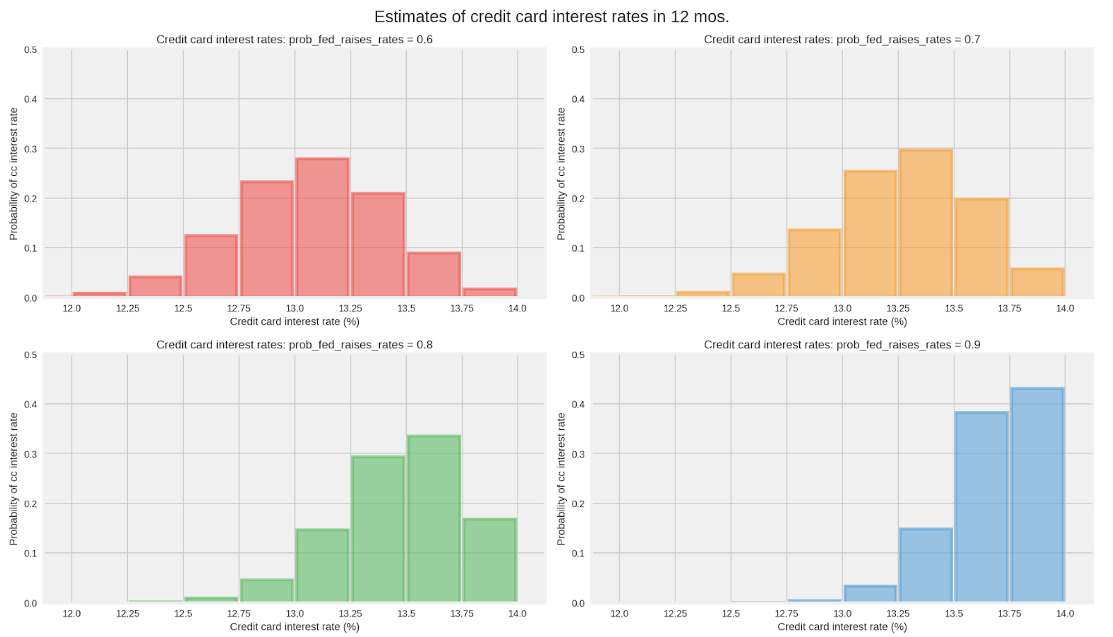
In the graphs below, notice how the probability distribution for your credit card rate in twelve months depends critically on your estimate about the probability of the Fed raising rates at each of the eight meetings. You can see that for every increase of 0.1 in your estimate of the Fed raising rates at each meeting, the expected interest rate for your credit card in twelve months increases by about 0.2%.

Even if all market participants used the binomial distribution in their models, it’s easy to see how they could disagree about the future prime rate because of the differences in their estimate for
probs. Indeed, this parameter is hard to estimate. Many institutions have dedicated analysts, including previous employees of the Fed, analyzing the Fed’s every document, speech and event to try to estimate this parameter.
Recall that we assumed that this parameter
probs was constant in our model for each of the next eight Fed meetings. How realistic is that? Members of the Federal Open Market Committee (FOMC), the rate setting body, are not just a set of biased coins. They can and do change their individual biases based on how the economy changes over time. The assumption that the parameter
probs will be constant over the next twelve months is not only unrealistic but also risky.
3. Errors from the failure of a model to adapt to structural changes: The underlying data-generating stochastic process may vary over time — i.e. the process is not stationary ergodic. We live in a dynamic capitalist economy characterized by technological innovations and changing monetary and fiscal policies. Time-variant distributions for asset values and risks are the rule, not the exception. For such distributions, parameter values based on historical data are bound to introduce error into forecasts.
In our example above, if the economy were to show signs of slowing down, the Fed might decide to adopt a more neutral stance in its fourth meeting making you change your
probs parameter from 70% to 50% going forward. This change in your
probs parameter will in turn change the forecast of your credit card interest rate.
Sometimes the time-variant distributions and their parameters change continuously or abruptly as in the Mexican Peso Crisis. For either continuous or abrupt changes, the models used will need to adapt to evolving market conditions. A new functional form with different parameters might be required to explain and predict asset values and risks in the new regime.
Suppose after the fifth meeting in our example, the US economy is hit by an external shock — say a new populist government in Greece decides to default on its debt obligations. Now the Fed may be more likely to cut interest rates than to raise them. Given this structural change in the Fed’s outlook, we will have to change the binomial probability distribution in our model to a trinomial distribution with appropriate parameters.
Conclusions
Finance is not a precise predictive science like physics. Not even close. So let’s not treat academic theories and models of finance as if they were models of quantum physics.
All financial models, whether based on academic theories or data mining strategies, are at the mercy of the trinity of modeling errors. While this trifecta of errors can be mitigated with appropriate modeling tools, it cannot be eliminated. There will always be asymmetry of information and cognitive biases. Models of asset values and risks will change over time due to the dynamic nature of capitalism, human behavior, and technological innovation.
Financial models need a framework that quantifies the uncertainty inherent in predictions of time-variant stochastic processes. Equally importantly, the framework needs to update continually the model or its parameters — or both — based on materially new datasets. Such models will have to be trained using small datasets, since the underlying environment may have changed too quickly to collect a sizable amount of relevant data.
In the next blog post, we’ll discuss the desiderata for a modeling framework to quantify and model the uncertainty generated by the trinity of modeling errors in finance.
Acknowledgements
We thank the TensorFlow Probability team, especially Mike Shwe and Josh Dillon, for their help in earlier drafts of this blog post.
References
- The Money Formula by David Orrell and Paul Wilmott, Wiley, 2017
- Nobels For Nonsense by J.R. Thompson, L.S. Baggett, W.C. Wojciechowski, and E.E. Williams, Journal of Post Keynesian Economics, Fall 2006
- Model Error by Katerina Simons, New England Economic Review, November 1997
- Bayesian Risk Management by Matt Sekerke, Wiley, 2015
