https://blog.tensorflow.org/2018/12/predicting-known-unknowns-with-tensorflow-probability-part2.html
https://blogger.googleusercontent.com/img/b/R29vZ2xl/AVvXsEjGUk7Lrysm0KEifTK8heUvqKbJLGNrPuRAEgLg9mCtUtoWpusFo5vMtfPqyy0OAxvo3iglsvooNT14HWzVsUsL22obX8xmrQy809L_z1JkgunbNbCr2aKLY-2unmvT42IfcnxmTqx3Wes/s1600/crackmeasurementsxsize.png
Posted by Venkatesh Rajagopalan, Director Data Science & Analytics and Arun Subramaniyan, VP Data Science & Analytics at BHGE Digital
In the
first blog of this series, we presented our analytics philosophy of combining domain knowledge, probabilistic methods, traditional machine learning (ML) and deep learning techniques to solve some of the hardest problems in the industrial world. We also illustrated this approach through an example of building a hybrid model for crack propagation. Our continued collaboration with the
TensorFlow Probability (TFP) team and the Cloud ML teams at Google has accelerated our journey to develop and deploy these techniques at scale. Previously intractable problems can now be solved by combining physics knowledge with seemingly unrelated techniques, deploying them with modern, scalable software and hardware.
In this blog, we will demonstrate another application of our analytics methodology — updating an existing model with newly available information. We will use the same example of crack propagation provided in the book
Prognostics and Health Management of Engineering Systems: An Introduction.
The Need for Updating Models
Prognostic models are built to make predictions on the future state of a system. These prognostic models can be completely data-driven, based on known physics of the system, or can be hybrid — a combination of both data and physics. In the industrial world, such models are used for estimating the remaining useful life of components (e.g., a turbine blade) or systems (e.g., an electrical submersible pump). These models can be developed using real-world, field data, if available, or with data from simulations or controlled experiments.
Models developed from simulations or controlled experiments need to be validated and refined with field data when they become available. However, re-building models with field data alone, when it becomes available, is generally not feasible since field data is usually very limited in quantity at a given time. Also, it is often desired to retain the model “kernel”, modifying only its coefficients. Thus, there exists a requirement for a methodology that allows for continuously updating models to improve their accuracy.
We will consider the following scenario: An initial model for crack propagation was built based on knowledge of physics and known material properties, as we did in the first blog. When this model was used to predict crack size, the model predictions were reasonably accurate for an initial period, but significant discrepancies were observed between predictions and observations over time.
Therefore, it would be useful to utilize the newly available crack measurements to update the existing model to make it more accurate.Such a scenario is quite common in the industrial domain; when material properties are altered or a new design is introduced in a component (e.g., blade of a gas turbine), there will be no field data available. This article discusses an approach based on the Unscented Kalman Filter (UKF) to update the initial crack propagation model.
A brief discussion on the Data
The data set, consisting of crack measurements and cycles, provided in
Prognostics and Health Management of Engineering Systems: An Introduction is depicted below:
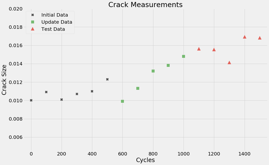
Though this data is from a textbook example, it exhibits certain characteristics that are commonly observed in field data such as the following:
1. Noise
While the overall trend in crack size with respect to cycles is increasing, it’s not strictly monotonic. At certain instances, the observed crack is less than what was measured at the previous instant. This may very well be due to measurement error, a common feature in field data. In other words, the data is noisy.
2. Small sample size
The data set consists of merely 16 data points, which is inadequate to build any meaningful data-driven model. Hence, it is critical to leverage the understanding of the physics of crack propagation in order to build a useful model.
To complicate things a bit further, in real-world applications, it may not even be possible to obtain data of progressive degradation from the same component or system. The data available for modeling is usually from different assets at various stages of degradation. Therefore, hybrid modeling approaches are critical for industrial analytics.
To illustrate an approach for updating models, the data set is divided into three parts:
- Initial data set — The initial model predictions are reasonably accurate in this data set. It consists of the first six data points [cycles 0 to 500].
- Update data set — The initial model predictions are not accurate in this data set. This data set, as the name suggests, is used to update the initial model. It consists of the next five data points [cycles 600 to 1000].
- Test data set — This data set is used to validate the predictions of the updated model. It consists of the last five data points [cycles 1100 to 1500]
The initial model parameters obtained using a least-squares minimization are
logC = -22.135 &
m = 3.765, where
C and
m are material properties. The model predictions, for the initial data set, are shown below:

The model predictions are fairly accurate with respect to the measured values. The mean squared error (MSE) for the initial data set is found to be: MSE(i)=3.93 10^-7.
The model’s prediction of crack sizes over the time-period corresponding to the update data set is shown below.

Clearly, the initial model’s predictions are no longer accurate. The MSE on the update data points becomes MSE(u)=5.67 10^-6, almost 14 times larger than the initial error, MSE(i)! Further, there’s a clear divergence between model predictions and the observed crack size in the update data set, as cycles increase. Therefore, the model needs to be refined to make it more accurate.
Update Methodology
One of the techniques that can be used for model updating is the
Kalman Filter (KF) and its variants, namely the
Extended Kalman Filter (EKF) and the
Unscented Kalman Filter (UKF).
The following assumptions are made in the case of KF:
- The process model is linear
- The measurement model is linear
- The initial state is Gaussian
The EKF and the UKF allow for the relaxation of the first two assumptions. A central operation performed in the Kalman Filter is the propagation of a Gaussian random variable (GRV) through the system dynamics. In the EKF, the state distribution is approximated by a GRV, which is then propagated analytically through the first-order linearization of the nonlinear system. This propagation can introduce large errors in the true posterior mean and covariance of the transformed GRV, which may lead to sub-optimal performance and sometimes divergence of the filter.
The UKF addresses this problem by using a deterministic sampling approach. The state distribution is again approximated by a GRV, but is now represented using a minimal set of carefully chosen sample points, called sigma points. When the sigma points are propagated through a nonlinear system, they capture the posterior mean and covariance
accurately to the 3rd order (Taylor series expansion) for any nonlinearity. In contrast, the EKF achieves only first-order accuracy. Remarkably, the computational complexity of the UKF is of the same order as that of the EKF.
As mentioned previously, we will utilize the UKF to update the initial crack propagation model. To do so, the problem needs to be cast in the UKF framework. The parameters that need to be updated,
C and
m, are considered as the “states” of the the UKF. By convention, the states are denoted by
x. The states are modeled as a random walk process. The crack propagation model, described earlier, is the measurement equation. Together, the process and measurement models of the UKF are represented as:

where
a is the crack size,
u is the number of cycles,
h represents the crack propagation model,
w is the process noise, and
v is the measurement noise. The process noise and measurement noise are assumed to be zero-mean, Gaussian and
white.
The steps in the UKF-based model-update methodology are summarized below:
- Initialize the state vector and its uncertainty (covariance).
- Generate sigma points based on the state.
- Propagate sigma points and compute predicted mean and covariance of the state.
- Compute sigma points based on predicted mean and covariance.
- Calculate output for each sigma point.
- Calculate the predicted output as the weighted sum of individual outputs from step 5.
- Calculate the uncertainty (covariance) of the predicted output.
- Compute the cross covariance between the predicted state and the predicted output.
- Compute the innovation as the difference between the measured output and the predicted output.
- Compute the filter gain using the cross covariance and output covariance.
- Update the state vector and its covariance.
- Repeat steps 2 to 11 for all the data points used for the model updating.
A curious reader can learn about the math behind the UKF,
here.
The UKF-based methodology for updating the crack propagation model has been implemented as a
Depend On Docker project and can be found in this
repository, with the Google Colab
here. Snippets of code for a few key steps of the algorithm are provided below for clarity.
Generate Sigma Points
The sigma points can be generated in TensorFlow using the following code:
## Inputs: State Vector - x_prev, Covariance Matrix - cov_prev, # States - num_st, UKF Parameter - kappa
## Output: Sigma Points Matrix - sig

[eigval, eigvec] = tf.linalg.eigh(cov_prev)                                   # Eigen Decomposition of the covariance matrix
S_tf = tf.diag(tf.sqrt(eigval))
sqrt_cov = tf.matmul(tf.matmul(eigvec, S_tf), tf.matrix_inverse(eigvec))      # Square-root of the covariance matrix
eta = tf.sqrt((alpha ** 2) * (num_st + kappa))                                # UKF scaling factor
sqrt_sc = tf.scalar_mul(eta, sqrt_cov)                                        # Scaled square-root
sig = np.matlib.repmat(x_prev, 1, 2*num_st+1)
sig[:, 1:num_st+1] = sig[:, 1:num_st+1] + sqrt_sc
sig[:, num_st+1:2*num_st+1] = sig[:, num_st+1:2*num_st+1] - sqrt_sc           # Sigma points
Predict Mean and Covariance
Once the sigma points are generated, they are propagated through the process model. The propagated sigma points are then used for the calculation of the predicted mean and covariance.
## Inputs:  Sigma Point Matrix - sig, UKF Weights - w0_mean, w0_cov, wi, # States - num_st, Process covariance - Q
## Outputs: Predicted State Vector - x_minus, Predicted Covariance - cov_minus

x_minus = w0_mean * sig[:, 0] + w_i * tf.reduce_sum(sig[:, 1:2 * num_st + 1], axis=1)
x_minus = tf.reshape(x_minus, (num_st, 1))
temp1 = tf.reshape(sig[:, 0], (num_st, 1))
# Predict Covariance
cov_minus = w0_cov * (temp1 - x_minus) * tf.transpose((temp1 - x_minus))
for i in range(1, 2 * num_st + 1):
  temp1 = tf.reshape(sig[:, i], (num_st, 1))
  cov_minus = cov_minus + w_i * (temp1 - x_minus) * tf.transpose((temp1 - x_minus))
  cov_minus = cov_minus + Q
Calculate Output for all Sigma Points
The outputs for all the sigma points are calculated as:
## Inputs: Sigma Point Matrix - sig, Current Crack Size - init_crack, Stress Constant - dsig,
##         Cycles Interval - diff_cycles, # States - num_st
## Output: Output Matrix - gam

gam = np.zeros((1, 2*num_st+1))
for indx in range(0, 2*num_st+1):
  logC = sig[0, indx]
  m = sig[1, indx]
  gam[:, indx] = predict_crack(diff_cycles, logC, m, init_crack, dsig)
Compute Output, Cross Covariance, and Output Covariance
The predicted output, cross and output covariances are calculated as follows:
## Inputs:  Output Matrix - gam, Sigma Point Matrix - sig, State Vector - x_prev, UKF Parameters - w0_mean, w0_cov, wi,
##          # States - num_st, Measurement Covariance - R
## Outputs: Cross Covariance - cov_xy, Output Covariance - cov_yy, Output Vector - yhat

yhat = w0_mean * gam[:, 0] + w_i * tf.reduce_sum(gam[:, 1:2 * num_st + 1])            # Output vector
temp2 = tf.reshape(sig[:, 0], (num_st, 1))
cov_yy = w0_cov * (gam[:, 0] - yhat) * tf.transpose(gam[:, 0] - yhat)                 # Output covariance
cov_xy = w0_cov * (temp2 - x_prev) * tf.transpose(gam[:, 0] - yhat)                   # Cross covariance
for i in range(1, 2*num_st+1):
  temp2 = tf.reshape(sig[:, i], (num_st, 1))
  cov_yy = cov_yy + w_i * (gam[:, i] - yhat) * tf.transpose(gam[:, i] - yhat)
  cov_xy = cov_xy + w_i * (temp2 - x_prev) * tf.transpose(gam[:, i] - yhat)

cov_yy = (cov_yy + tf.transpose(cov_yy))/2                                            # Ensure symmetry
cov_yy = cov_yy + R
Update State Vector and its Covariance
Finally, the state vector and its covariance are updated.
## Inputs : Predicted State Vector - x_minus, Predicted State Covariance - cov_minus, Predicted Output - yhat,
#           Measured Output - y, Output Covariance cov_yy, Cross Covariance - cov_xy
## Outputs: Updated State Vector - x_hat, Updated State Covariance - cov_hat

k_gain = cov_xy * np.linalg.inv(np.matrix(cov_yy))                            # calculate filter gain
innov = y - y_hat                                                             # innovation
x_hat = x_minus + k_gain * innov                                              # update state
cov_hat = cov_minus - k_gain * cov_yy * tf.transpose(k_gain)                  # update covariance
cov_hat = (cov_hat + tf.transpose(cov_hat)) / 2                               # ensure symmetry
Results and Discussion
As mentioned earlier, the update data set was used to refine the initial model using the UKF. The model parameters, after updating, were found to be:
logC = -22.2037 &
m = 3.5762. The predictions, before and after model update, are presented below:

It can be observed that the updated model predictions are more accurate when compared with the initial model. But, this is a rather obvious result, as we are predicting on the same data set that was used for updating the model. The accuracy of the updated model can be truly gauged only if its predictions are validated on a data set that wasn’t used for the update. More importantly, the updated model should be more accurate than the initial model in predicting the future evolution of the crack. Otherwise, even the updated model is not particularly useful.
Accordingly, the updated model was used to predict the crack sizes for cycles corresponding to the test data set. The crack sizes, predicted by the updated model along with those of the initial model are shown below:

The UKF based model update methodology not only estimates the mean of the model parameters, but also computes the covariance associated with the estimates. In other words, it provides the joint distribution of the state variables. TensorFlow Probability’s
MultivariateNormalFullCovariance function is utilized to create samples for computing the uncertainty associated with the predicted output, which in this case is the crack size. The 95% credible interval of the predicted crack size is also plotted in the figure above.
From the plot, it is clear that the updated model is significantly more accurate at predicting the future evolution of the crack, when compared to the initial model. This suggests that UKF has been able to extract pertinent information from the measurements in the Update data set to modify the model parameters to make the model more accurate and useful. Another important thing to note here is the robustness of this approach to noisy measurements. In the update data set, measurements corresponding to cycles 600 and 700 are outliers when compared to other measured values of crack. However, the impact of these outliers on the model update process is rather minimal as the UKF didn’t try to minimize the error between the predictions and observations at these data points. This is a desirable outcome and such robustness to noisy measurements is critical for obtaining an accurate updated model.
Finally, we forecast the crack size to 2200 cycles with both the initial model and the updated model. The predictions along with the uncertainty bounds of the updated model are shown below.

It is obvious from the chart above that the crack predictions would have been highly inaccurate if the initial model were used. In fact, the initial model would have led to a false alarm being generated at 2100 cycles, when the true chance of finding a crack greater than the repair threshold is significantly small (<< 5 %).
Summary
We have shown how to address the issue of “known unknowns”, as we described in
Part 1 of this blog series. In Part 1, we showed how to combine the domain knowledge and traditional ML to compute the known knowns of material properties. The same example in a more real-world setting where all the data is not available upfront was shown here. The UKF-based methodology for updating prognostic models, discussed in this blog, can be very effective in real-world applications where the data is limited and noisy. It can accommodate non-linearities in the model and is computationally efficient.
Next steps
As we build on the concepts from
Part 1, we have expanded the known knowns problem to the known unknowns in Part 2. The next part will address the case of unknown unknowns, bringing all the three pieces together. Several open questions around Bayesian model selection and model optimization will be addressed in future blogs.
Acknowledgments
This blog is a result of the hard work and deep collaboration of several teams at Google and BHGE. We are particularly grateful to Josh Dillon,
Mike Shwe, Scott Fitzharris, Alex Walker, Shyam Sivaramakrishnan, and Fabio Nonato for their many edits, results, code snippets, and — most importantly — enthusiastic support


