Regression with Probabilistic Layers in TensorFlow Probability
mars 12, 2019
Posted by Pavel Sountsov, Chris Suter, Jacob Burnim, Joshua V. Dillon, and the TensorFlow Probability team

TensorFlow Probability

Background

At the 2019 TensorFlow Dev Summit, we announced Probabilistic Layers in TensorFlow Probability (TFP). Here, we demonstrate in more detail how to use TFP layers to manage the uncertainty inherent in regression predictions.

Regression and Probability

Regression is one of the most basic techniques that a machine learning practitioner can apply to prediction problems However, many analyses based on regression omit a proper quantification of the uncertainty in the predictions, owing partially to the degree of complexity required. To start to quantify the uncertainty, a particularly elegant way of posing the problem is to write the regression model as P(y | x, w), the probability distribution of labels (y), given the inputs (x) and some parameters (w). We can fit this model to the data by maximizing the probability of the labels, or equivalently, minimizing the negative log-likelihood loss: -log P(y | x). In Python:
negloglik = lambda y, p_y: -p_y.log_prob(y)
We can use a variety of standard continuous and categorical and loss functions with this model of regression. Mean squared error loss for continuous labels, for example, means that P(y | x, w) is a normal distribution with a fixed scale (standard deviation). Cross-entropy loss for classification means that P(y | x, w) is the categorical distribution.

In this post we will show how to use probabilistic layers in TensorFlow Probability (TFP) with Keras to build on that simple foundation, incrementally reasoning about progressively more uncertainty of the task at hand. You can follow along in this Google Colab.

Case 1: Simple Linear Regression

We shall begin with a simple linear regression model fit to some data:
import tensorflow as tf
import tensorflow_probability as tfp
tfd = tfp.distributions

# Build model.
model = tf.keras.Sequential([
  tf.keras.layers.Dense(1),
  tfp.layers.DistributionLambda(lambda t: tfd.Normal(loc=t, scale=1)),
])

# Do inference.
model.compile(optimizer=tf.optimizers.Adam(learning_rate=0.05), loss=negloglik)
model.fit(x, y, epochs=500, verbose=False)

# Make predictions.
yhat = model(x_tst)
The inference and prediction sections should be familiar to anyone who has used Keras before, but the model construction will look different. We make it explicit that we’re modeling the labels using a normal distribution with a scale of 1 centered on location (mean) that’s dependent on the inputs. The tfp.layers.DistributionLambda layer in fact returns a special instance of tfd.Distribution (see Appendix A for more details about this), so we are free to take its mean and plot it next to the data:
mean = yhat.mean()
the overall trend of the data (blue circles) with the predicted mean of the distribution over labels
Thus, we managed to capture the overall trend of the data (blue circles) with the predicted mean of the distribution over labels. However, we can see that the data has more structure: it appears that the y gets more variable as x increases. The model we’ve written so far cannot capture this detail, but in the next section we’ll show how we can modify the model to give it that ability.

Case 2: Known Unknowns

In the previous section we’ve seen that there is variability in y for any particular value of x. We can treat this variability as being inherent to the problem. This means that even if we had an infinite training set, we still wouldn’t be able to predict the labels perfectly. A common example of this kind of uncertainty is the outcome of a fair coin flip (assuming you are not equipped with a detailed model of physics etc.). No matter how many flips we’ve seen in the past, we cannot predict what the flip will be in the future.

We will assume that this variability has a known functional relationship to the value of x. Let us model this relationship using the same linear function as we did for the mean of y.
# Build model.
model = tfk.Sequential([
  tf.keras.layers.Dense(1 + 1),
  tfp.layers.DistributionLambda(
      lambda t: tfd.Normal(loc=t[..., :1],
                           scale=1e-3 + tf.math.softplus(0.05 * t[..., 1:]))),
])

# Do inference.
model.compile(optimizer=tf.optimizers.Adam(learning_rate=0.05), loss=negloglik)
model.fit(x, y, epochs=500, verbose=False)

# Make predictions.
yhat = model(x_tst)
Now, in addition to predicting the mean of the label distribution, we also predict its scale (standard deviation). After training and forming the predictions the same way, we can get meaningful predictions about the variability of y as a function of x. Like before:
mean = yhat.mean()
stddev = yhat.stddev()
mean_plus_2_stddev = mean - 2. * stddev
mean_minus_2_stddev = mean + 2. * stddev
new model graph
Much better! Our model is now less certain about what y should be as x gets larger. This kind of uncertainty is called aleatoric uncertainty, because it represents variation inherent to the underlying process . Though we’ve made progress, aleatoric uncertainty is not the only source of uncertainty in this problem. Before going further, let us consider the other source of uncertainty that we’ve hitherto ignored.

Case 3: Unknown Unknowns

The noise in the data means that we can not be fully certain of the parameters of the linear relationship between x and y. For example, the slope we’ve found in the previous section seems reasonable, but we don’t know for sure, and perhaps a slightly shallower or steeper slope would also be reasonable. This kind of uncertainty is called the epistemic uncertainty; unlike aleatoric uncertainty, epistemic uncertainty can be reduced if we get more data. To get a sense of this uncertainty we shall replace the standard Keras 
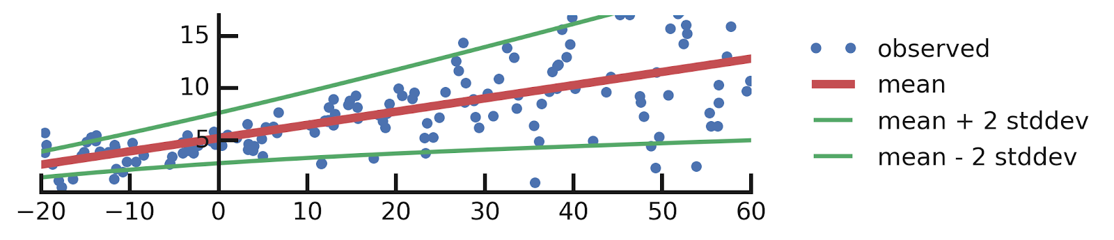
Dense layer with TFP’s DenseVariational layer.

The DenseVariational layer uses a variational posterior Q(w) over the weights to represent the uncertainty in their values. This layer regularizes Q(w) to be close to the prior distribution P(w), which models the uncertainty in the weights before we look into the data.

For Q(w) we’ll use a multivariate normal distribution for the variational posterior with a trainable diagonal covariance matrix centered on a trainable location. For P(w) we’ll use a standard multivariate normal distribution for the prior with a trainable location and fixed scale. See Appendix B for more details about how this layer works.

Let’s put that all together:
# Build model.
model = tf.keras.Sequential([
  tfp.layers.DenseVariational(1, posterior_mean_field, prior_trainable),
  tfp.layers.DistributionLambda(lambda t: tfd.Normal(loc=t, scale=1)),
])

# Do inference.
model.compile(optimizer=tf.optimizers.Adam(learning_rate=0.05), loss=negloglik)
model.fit(x, y, epochs=500, verbose=False)

# Make predictions.
yhats = [model(x_tst) for i in range(100)]
Despite the complexity of the algorithms involved, using the DenseVariational layer is simple. One interesting aspect of the code above is that when we make predictions using a model with such a layer, we get a different answer every time we do so. This is because DenseVariational essentially defines an ensemble of models. Let us see what this ensemble tells us about the parameters of our model.
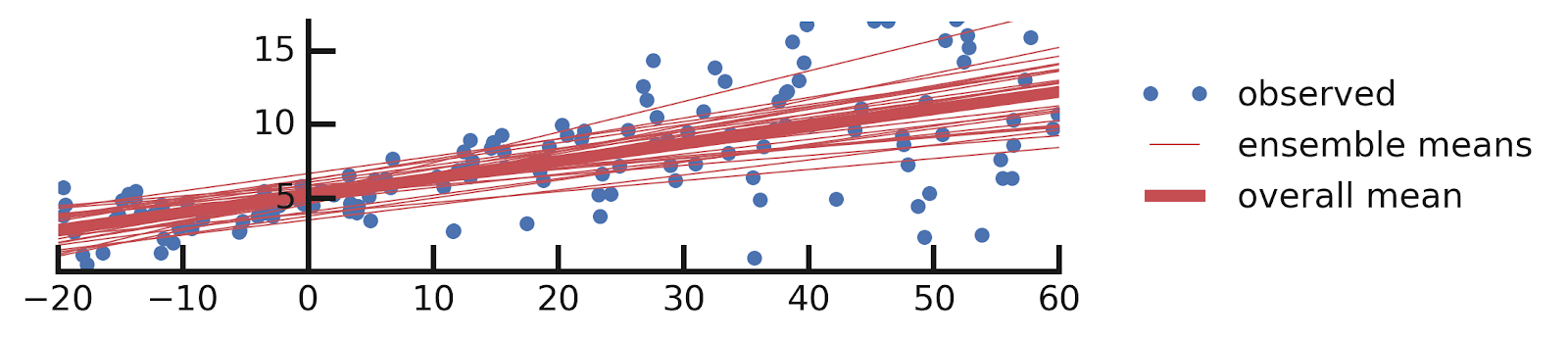
Graph with random draw of model parameters
Each line represents a different random draw of the model parameters from the posterior distribution. As we can see, there is in fact quite a bit of uncertainty about the linear relationship. Even if we don’t care about the variability of y for any particular value of x, the uncertainty in the slope should give us pause if we’re making predictions for x’s too far from 0.

Note that in this example we are training both P(w) and Q(w). This training corresponds to using Empirical Bayes or Type-II Maximum Likelihood. We used this method so that we wouldn’t need to specify the location of the prior for the slope and intercept parameters, which can be tough to get right if we do not have prior knowledge about the problem. Moreover, if you set the priors very far from their true values, then the posterior may be unduly affected by this choice. A caveat of using Type-II Maximum Likelihood is that you lose some of the regularization benefits over the weights. If you wanted to do a proper Bayesian treatment of uncertainty (if you had some prior knowledge, or a more sophisticated prior), you could use a non-trainable prior (see Appendix B).

Case 4: Known and Unknown Unknowns

Now that we looked at aleatoric and epistemic uncertainty in isolation, we can use TFP layers’ composable API to create a model that reports both types of uncertainty:
# Build model.
model = tf.keras.Sequential([
  tfp.layers.DenseVariational(1 + 1, posterior_mean_field, prior_trainable),
  tfp.layers.DistributionLambda(
      lambda t: tfd.Normal(loc=t[..., :1],
                           scale=1e-3 + tf.math.softplus(0.01 * t[..., 1:]))),
])

# Do inference.
model.compile(optimizer=tf.optimizers.Adam(learning_rate=0.05), loss=negloglik)
model.fit(x, y, epochs=500, verbose=False);

# Make predictions.
yhats = [model(x_tst) for _ in range(100)]
The only change we’ve made to the previous model is that we added an extra output to DenseVariational layer to also model the scale of the label distribution. As in our previous solution, we get an ensemble of models, but this time they all also report the variability of y as a function of x. Let us plot this ensemble:

Note the qualitative difference between the predictions of this model compared to those from the model that considered only aleatoric uncertainty: this model predicts more variability as x gets more negative in addition to getting more positive — something that is not possible to do with a simple linear model of aleatoric uncertainty.

Conclusion

The guiding principle behind TFP layers is that the practitioner should focus on writing models, not losses. Throughout this post we have kept the user-specified loss the same, the negloglik function that implements the negative log-likelihood, while making local alterations to the model to handle more and more types of uncertainty. The API also lets you freely switch between Maximum Likelihood learning, Type-II Maximum Likelihood and and a full Bayesian treatment. We believe that this API significantly simplifies construction of probabilistic models and are excited to share it with the world.

This API will be ready to use in the next stable release, TensorFlow Probability 0.7.0, and is already available in the nightly version. Please join us on the tfprobability@tensorflow.org forum for the latest TensorFlow Probability announcements and other TFP discussions.

Bonus: Tabula Rasa

So far we’ve been assuming that the data follows a line. What if we don’t know the functional relationship between the inputs and the labels? Suppose we have a vague sense that the predicted labels should be similar to the labels already seen only if the corresponding inputs are close to what we’ve already observed? In other words, the only assumption we wish to make is that the function we’re fitting to the data is smooth.

The standard tool for doing regression while making these sorts of assumptions is the Gaussian Process. This powerful model uses a kernel function to encode the smoothness assumptions (and other global function properties) about what form the relationship between the inputs and labels should take. Conditioned on the data, it forms a probability distribution over functions that are consistent with those assumptions and the data.

TFP provides the VariationalGaussianProcess layer, which uses a variational approximation (similar in spirit to what we did in case 3 and 4 above) to a full Gaussian Process for an efficient yet flexible regression model. For simplicity, we’ll be considering only the epistemic uncertainty about the form of the relationship between inputs and labels. In terms of the assumptions we’ll be making, we’ll simply assume that the function we’re fitting is locally smooth: it can vary as much as it wants across the entire dataset, but if two inputs are close, it’ll return similar values.
num_inducing_points = 40
model = tf.keras.Sequential([
    tf.keras.layers.InputLayer(input_shape=[1], dtype=x.dtype),
    tf.keras.layers.Dense(1, kernel_initializer='ones', use_bias=False),
    tfp.layers.VariationalGaussianProcess(
        num_inducing_points=num_inducing_points,
        kernel_provider=RBFKernelFn(dtype=x.dtype),
        event_shape=[1],
        inducing_index_points_initializer=tf.constant_initializer(
            np.linspace(*x_range, num=num_inducing_points,
                        dtype=x.dtype)[..., np.newaxis]),
        unconstrained_observation_noise_variance_initializer=(
            tf.constant_initializer(
                np.log(np.expm1(1.)).astype(x.dtype))),
    ),
])

# Do inference.
batch_size = 32
loss = lambda y, rv_y: rv_y.variational_loss(
    y, kl_weight=np.array(batch_size, x.dtype) / x.shape[0])
model.compile(optimizer=tf.optimizers.Adam(learning_rate=0.01), loss=loss)
model.fit(x, y, batch_size=batch_size, epochs=1000, verbose=False)

# Make predictions.
yhats = [model(x_tst) for _ in range(100)]
Due to its power, the definition of this model is significantly more complex: we need to define a new loss function, and there are more parameters to specify. In the near future, the TFP team will be working to simplify this model further. This added complexity is worth it, however, as evidenced by the results:

The VariationalGaussianProcess has discovered a periodic structure in the training set! Indeed, that structure was present in the data used throughout this post all along — did you notice it before the model did? Importantly, the model discovered this structure without us telling it that there was any such periodicity in the data. And, as advertised, it is still giving us a measure of uncertainty. For example, close to 0, the periodic structure is not as apparent, so the model does not commit to any such relationship in that region.

Appendix A: How does DistributionLambda work?

DistributionLambda is a special Keras layer that uses a Python lambda to construct a distribution conditioned on the layer inputs:
layer = tfp.layers.DistributionLambda(lambda t: tfd.Normal(t, 1.))
distribution = layer(2.)
assert isinstance(distribution, tfd.Normal)
distribution.loc
# ==> 2.
distribution.stddev()
# ==> 1.
This layer enables us to write the negloglik loss function as we did, because Keras passes the output of the final layer of the model into the loss function, and for the models in this post, all those layers return distributions. See the Variational Autoencoders with Tensorflow Probability Layers post for more ways to use these layers.

Appendix B: How does DenseVariational work?

The DenseVariational layer enables learning a distribution over its weights using variational inference. This is done by maximizing the ELBO (Evidence Lower BOund) objective:
ELBO formula
ELBO uses three distributions:
  • P(w) is the prior over the weights. It is the distribution we assume the weights to follow before we trained the model.
  • Q(w; θ) is the variational posterior parameterized by parameters θ. This is an approximation to the distribution of the weights after we have trained the model.
  • P(Y | X, w) is the likelihood function relating all inputs X, all labels Y and the weights. When used as a probability distribution over Y, it specifies the variation in Y given X and the weights.
ELBO is a lower bound on log P(Y | X), i.e. the log-likelihood of the labels given the inputs after marginalizing away the uncertainty over the weights. ELBO works by trading off the KL divergence of Q with respect to the prior over the weights (the second term), with the ability to predict labels from the inputs (the first term). When there is little data, the second term dominates and our weights remain close to the prior distribution, which as a side effect helps prevent overfitting.

DenseVariational computes the two terms of the ELBO separately. The first term is computed by approximating it with a single random sample from Q. If we look at that term closely, then for any specific value of w it is exactly the negative log-likelihood loss we’ve been using for regression in this post. Thus, by simply drawing a random set of weights from Q and then computing the regular loss, we automatically approximate the first term of ELBO.

The second term is computed analytically, and then added to the layer as a regularization loss — similar to how we’d specify something like an L2 regularization. This loss is added to the first term for us by Keras.

The sampling used to computed the first term explains how we were able to generate multiple models by calling the model with the same inputs multiple times: each time we did that, we sampled a new set of weights according to the Q distribution

How do we specify the prior and the variational posterior? They’re trainable distributions just like we’ve seen in the case 2. For example, the trainable prior we used in case 3 is defined as follows:
def prior_trainable(kernel_size, bias_size=0, dtype=None):
  n = kernel_size + bias_size
  return tf.keras.Sequential([
      tfp.layers.VariableLayer(n, dtype=dtype),
      tfp.layers.DistributionLambda(lambda t: tfd.Independent(
          tfd.Normal(loc=t, scale=1),
          reinterpreted_batch_ndims=1)),
  ])
It’s just a callable that returns a regular Keras model with a DistributionLambda layer! The only new component here is the VariableLayer which simply returns the value of a trainable variable, ignoring any inputs (because the prior is not conditioned on any inputs). Note that if we wanted to convert this to a non-trainable prior, we would pass trainable=False to VariableLayer constructor.
Next post
Regression with Probabilistic Layers in TensorFlow Probability

Posted by Pavel Sountsov, Chris Suter, Jacob Burnim, Joshua V. Dillon, and the TensorFlow Probability team


BackgroundAt the 2019 TensorFlow Dev Summit, we announced Probabilistic Layers in TensorFlow Probability (TFP). Here, we demonstrate in more detail how to use TFP layers to manage the uncertainty inherent in regression predictions.
Regression and ProbabilityRegression is one of the most basic …