https://blog.tensorflow.org/2019/06/high-performance-inference-with-TensorRT.html?hl=es
https://blogger.googleusercontent.com/img/b/R29vZ2xl/AVvXsEiHjIkv1Vlk4qdElzt213yRP7MSM8pYxUcHqzpdv43P3b9wIHEgqXL18TvfvWG1xqCK3kA9ANSpd8_fIg9TqNisiJ7C4_pkRzHiQ_BirrLSjnwmfdxdFP7XKVC0rArfJT3KuONOrNYg5zE/s1600/fig1a.png
Posted by Pooya Davoodi (NVIDIA), Guangda Lai (Google), Trevor Morris (NVIDIA), Siddharth Sharma (NVIDIA)
Last year we
introduced integration of TensorFlow with TensorRT to speed up deep learning inference using GPUs. This article dives deeper and share tips and tricks so you can get the most out of your application during inference. Even if you are unfamiliar with the integration, this article provides enough context so you can follow along.
By the end of this article, you will know:
- Models supported and integration workflow
- New techniques such as quantization aware training to use with INT8 precision
- Profiling techniques to measure performance
- New experimental features and a peek at the roadmap
Three Phases of Optimization with TensorFlow-TensorRT
Once trained, a model can be deployed to perform inference. You can find several pre-trained deep learning models on the
TensorFlow GitHub site as a starting point. These models use the latest TensorFlow APIs and are updated regularly. While you can run inference in TensorFlow itself, applications generally deliver higher performance using TensorRT on GPUs. TensorFlow models optimized with TensorRT can be deployed to T4 GPUs in the datacenter, as well as Jetson Nano and Xavier GPUs.
So what is TensorRT?
NVIDIA TensorRT is a high-performance inference optimizer and runtime that can be used to perform inference in lower precision (FP16 and INT8) on GPUs. Its integration with TensorFlow lets you apply TensorRT optimizations to your TensorFlow models with a couple of lines of code. You get up to 8x higher performance versus TensorFlow only while staying within your TensorFlow environment. The integration applies optimizations to the supported graphs, leaving unsupported operations untouched to be natively executed in TensorFlow. The latest version of the integrated solution is always available in the
NVIDIA NGC TensorFlow container.
The integrated solution can be applied to models in applications such as object detection, translation, recommender systems, and reinforcement learning. Accuracy numbers for an expanding set of models including MobileNet, NASNet, Inception and ResNet
are available and updated regularly.
Once you have the integration installed and a trained TensorFlow model, export it in the saved model format. The integrated solution then applies TensorRT optimizations to the subgraphs supported by TensorFlow. The output is a TensorFlow graph with supported subgraphs replaced with TensorRT optimized engines executed by TensorFlow. The workflow and code to achieve the same are below:
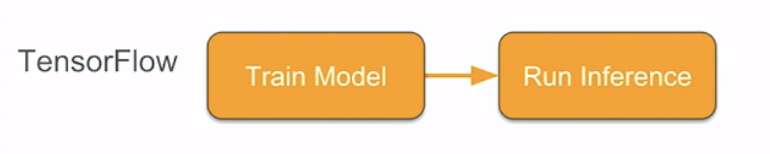
 |
| Fig 1 (a) workflows when performing inference in TensorFlow only and in TensorFlow-TensorRT using ‘savedmodel’ format |
import tensorflow.contrib.tensorrt as trt
trt.create_inference_graph(
    input_saved_model_dir = input_saved_model_dir,
    output_saved_model_dir = output_saved_model_dir)
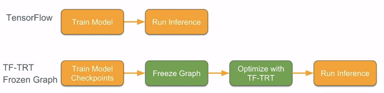 |
| Fig 1 (b) workflows when performing inference in TensorFlow only and using TensorFlow-TensorRT using frozen graphs |
Another approach to export the TensorFlow model for inference is to freeze the trained model graph for inference. The image and code snippet below shows how to apply TensorRT optimizations to a graph in TensorFlow when using this approach. The output is a TensorFlow graph with supported subgraphs replaced with TensorRT optimized engines that can then be executed by TensorFlow.
import tensorflow.contrib.tensorrt as trt
converted _graph_def = trt.create_inference_graph(
     input_graph_def = frozen_graph,
     outputs-[‘logits’, ‘classes’])
We maintain an
updated list of operations supported by the integrated workflow.
Three operations are performed in the optimization phase of the process outlined above:
- Graph partition.TensorRT scans the TensorFlow graph for sub-graphs that it can optimize based on the operations supported.
- Layer conversion. Converts supported TensorFlow layers in each subgraph to TensorRT layers.
- Engine optimization. Finally, subgraphs are then converted into TensorRT engines and replaced in the parent TensorFlow graph.
Let’s look at an example of this process.
Example walkthrough
Take the graph below as an example. Green blocks highlight ops supported by TensorRT and gray blocks show an unsupported op (“Cast”).
The first phase of the optimization partitions the TensorFlow graph into TensorRT compatible versus non-compatible subgraphs. We traverse the graph backwards starting with the Relu operation (a) and add one node at a time to get to the largest subgraph possible. The only constraint is that the subgraph should be a direct cyclic graph and have no loops. The largest subgraph that can be created is shown in ©. The cluster adds all nodes till it gets to the
reshape op. Then there is a loop (d), so it goes back. We now add a new cluster for it, so we finally end with 2 TensorRT compatible subgraphs (e).
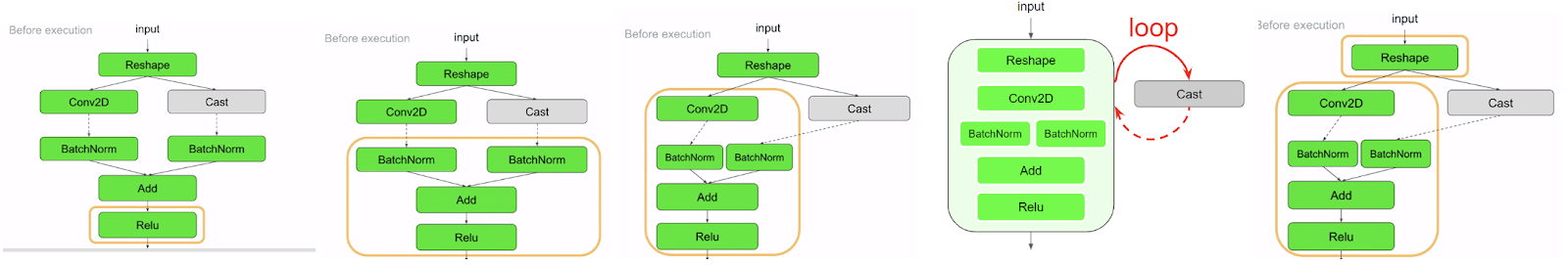
|
| Fig 2 (a) Example graph, TensorRT supported nodes in green, graph selected for optimization shown in orange box (b) 4 ops in the subgraph, no loops yet (c) adding Conv2D also does not add a loop (d) adding reshape to this subgraph creates a loop (e) 2 subgraphs created resolving the loop |
Controlling Minimum Number of Nodes in a TensorRT engine
In the example above, we generated two TensorRT optimized subgraphs: one for the
reshape operator and another for all ops other than
cast. Small graphs, such as ones with just a single node, present a tradeoff between optimizations provided by TensorRT and the overhead of building and running TRT engines. While small clusters might not deliver high benefit, accepting only very large clusters would leave possible optimizations that were applicable to smaller clusters on the table. You can control the size of subgraphs by using the
minimum_segment_size parameter. Setting this value to 3 (default value) would not generate TensorRT engines for subgraphs consisting of less than three nodes. In this example, a minimum segment size of 3 would skip having TensorRT optimize the reshape op even though it’s eligible for the TensorRT optimization, and will fall back to TensorFlow for the reshape op.
converted_graph_def = create_inference_graph(
    input_saved_model_dir=model_dir,
    minimum_segment_size=3,
    is_dynamic_op=True,
    maximum_cached_engines=1)
The final graph includes 2 subgraphs or clusters (Fig 3a).
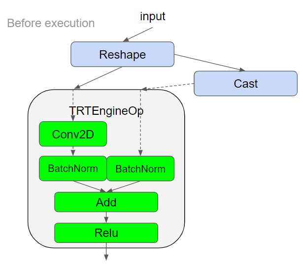 |
| Fig 3 (a) subgraph with TensorFlow operations (b) TensorFlow subgraph replaced with a TensorRTEngineOp. Next, the TensorRT compatible subgraph is wrapped into custom op called TRTEngineOp. The newly generated TensorRT op is then used to replace the TensorFlow subgraph. The final graph has 3 ops (Fig 3b). |
Variable Input Shapes
TensorRT usually requires that all shapes in your model are fully defined (i.e. not -1 or None, except the batch dimension) in order to select the most optimized CUDA kernels. If the input shapes to your model are fully defined, the default setting of
is_dynamic_op=False can be used to build the TensorRT engines statically during the initial conversion process. If your model does have unknown shapes for models such as BERT or Mask R-CNN, you can delay the TensorRT optimization to execution time when input shapes will be fully specified. Set
is_dynamic_op to
true to use this approach.
converted_graph_def = create_inference_graph(
    input_saved_model_dir=model_dir,
    minimum_segment_size=3,
    is_dynamic_op=false,
    maximum_cached_engines=1)
Next, the graph is traversed in topological order to convert each TensorFlow op in the subgraph to one or more TensorRT layers. And finally TensorRT applies optimizations such as layer and tensor fusion, calibration for lower precision, and kernel auto-tuning. These optimizations are transparent to the user and are optimized for the GPU that you plan to run inference on.
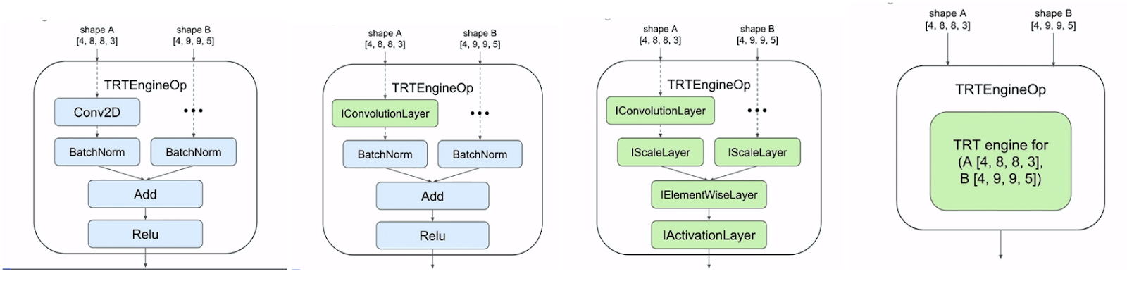
|
| Fig 4 (a) TensorFlow subgraph before conversion to TensorRT layers (b) first TensorFlow op is converted to TensorRT layer (c) All TensorFlow ops converted to TensorRT layers (d) final TensorRT engine from the graphs |
TensorRT Engine Cache and Variable Batch Sizes
TensorRT engines can be cached in an LRU cache located in the TRTEngineOp op. The key to this cache are the shapes of the op inputs. So a new engine is created if the cache is empty or if an engine for a given input shape does not exist in the cache. You can control the number of engines cached with the
maximum_cached_engines parameter as below.
converted_graph_def = create_inference_graph(
    input_saved_model_dir=model_dir
    minimum_segment_size=3,
    is_dynamic_op=True,
    maximum_cached_engines=1)
Setting the value to 1, will force any existing cache to be evicted each time a new engine is created.
TensorRT uses batch size of the inputs as one of the parameters to select the highest performing CUDA kernels. The batch size is provided as the first dimension of the inputs. The batch size is determined by input shapes during execution when
is_dynamic_op is
true, and by the
max_batch_size parameter when
is_dynamic_op is
false. An engine can be reused for a new input, if:
- engine batch size is greater than or equal to the batch size of new input, and
- non-batch dims match the new input
So in Fig 5a below, we do not need to create a new engine as the new batch size (2) is less than the batch size of the cached engine (4) while the other inputs dimension ([8,8,3] and [9,9,5] in this case) are the same. In 5b, the time non-batch size input dims are different ([8,8,3] vs [9,9,5]), and so a new engine will need to be generated. The final schematic representation of cache with the engines is shown in 5c.
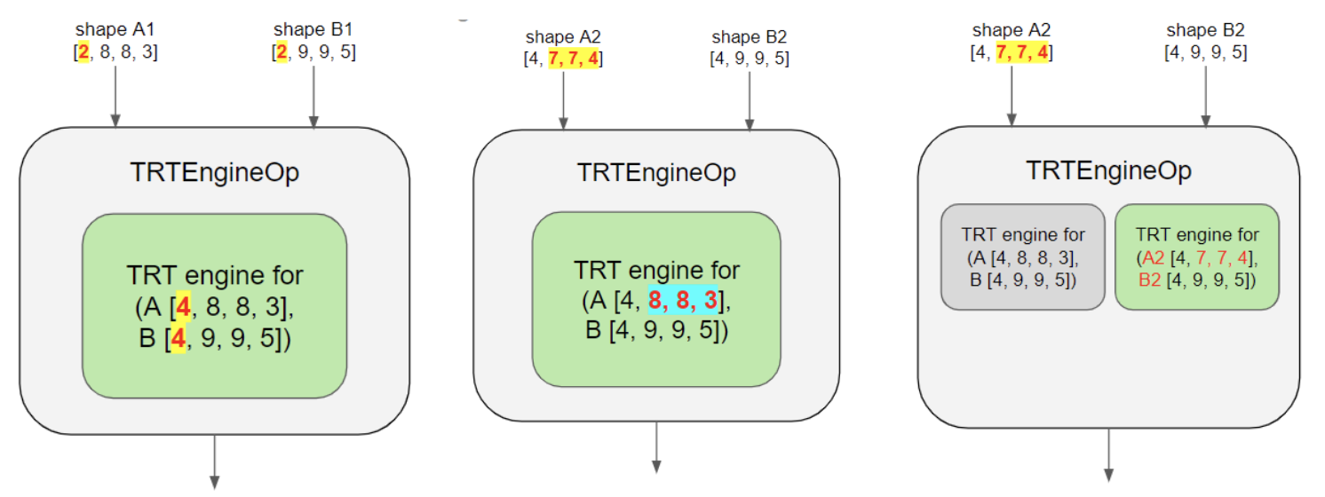
|
| Fig 5 (a), (b), (c) from left to right |
Increase the
maximum_cached_engines variable to prevent recreation of engines as much as possible. Caching more engines uses more resources on the machine, but we have not found that to be a problem for typical models.
Inference in INT8 Precision
Tesla T4 GPUs introduced Turing Tensor Core technology with a full range of precision for inference, from FP32 to FP16 to INT8. Tensor Cores deliver up to 30 teraOPS (TOPS) of throughput on the Tesla T4 GPUs. Using INT8 and mixed precision reduces the memory footprint, enabling larger models or larger mini-batches for inference.
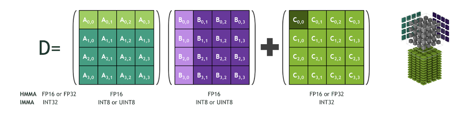
|
| Fig 6 Tensor Core performing matrix multiplication in reduced precision and accumulate in higher precision |
You might wonder how it is possible to take a model operating in 32 bit floating point precision, representing billions of different numbers, and reduce all of that to an 8 bit integer only representing 256 possible values. Typically, the values of weights and activations lie in some small range in deep neural networks. If we can focus our precious 8 bits just in that range, we can maintain good precision with just some small rounding error.
TensorRT uses “symmetric linear quantization” for quantization, a scaling operation from the FP32 range (which is -6 to 6 in Fig 7) to the INT8 range (which for us is -127 to 127 to preserve symmetry). If we can find the range where the majority of values lie for each intermediate tensor in the network, we can quantize that tensor using that range while maintaining good accuracy
Quantize(x, r) = round(s * clip(x, -r, r))
            where s = 127 / r
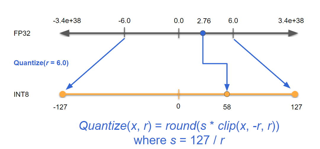
|
| Fig 7: x is the input, r is the floating point range for a tensor, s is the scaling factor for number of values in INT8. Equation above takes the input x and returns a quantized INT8 value. |
While an exhaustive treatment is out of scope for this article, two techniques are commonly used to determine activation ranges for each tensor in a network: calibration and quantization aware training.
Calibration is the recommended approach and works with most models with minimal accuracy loss (<1%). For calibration, inference is first run on a calibration dataset. During this calibration step, a histogram of activation values is recorded.The INT8 quantization ranges are then chosen to minimize information loss. Quantization happens late in the process, which becomes a new source of error for the training. See the code example below on how to perform calibration:
import tensorflow.contrib.tensorrt as trt
calib_graph = trt.create_inference_graph(…
    precision_mode=’INT8',
    use_calibration=True)
with tf.session() as sess:
    tf.import_graph_def(calib_graph)
    for i in range(10):
        sess.run(‘output:0’, {‘input:0’: my_next_data()})
# data from calibration dataset
converted_graph_def = trt.calib_graph_to_infer_graph(calib_graph)
When using calibration for INT8, the quantization step happens after the model has been trained. This means no way exists to adjust the model for the error at that stage. Quantization-aware training tries to address this, though this is still in its early stages and released as an experimental feature. Quantization aware training models the quantization error during a fine-tuning step of training and quantization ranges are learned during training. This allows your model to compensate for the error. This can provide better accuracy than calibration in some cases.
Augment the graph with quantization nodes and then train the model as normal to perform quantization aware training. The quantization nodes will model the error due to quantization by clipping, scaling, rounding, and unscaling the tensor values, allowing the model to adapt to the error. You can use fixed quantization ranges or make them trainable variables. You can use
tf.quantization.fake_quant_with_min_max_vars with
narrow_range=True and
max=min to match TensorRT’s quantization scheme for activations.
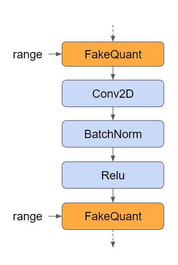 |
| Fig 8 Quantization nodes in orange inserted in the TensorFlow graph |
Other changes involve setting
precision_mode=”INT8” and
use_calibration=false as shown below:
calib_graph_def = create_inference_graph(
    input_saved_model_dir=input_saved_model_dir,
    precision_mode=”INT8",
    use_calibration=False)
This extracts the quantization range from the graph and gives you the converted model for inference. The error is modeled using fake quantization nodes, for each one the range can be learned using gradient descent. TF-TRT will automatically absorb the learned quantization ranges from your graph and will create an optimized INT8 model ready for deployment.
Note that INT8 inference must be modeled as closely as possible during training. This means that you must not introduce a TensorFlow quantization node in places that will not be quantized during inference (due to a fusion occurring). Operation patterns such as Conv > Bias > Relu or Conv > Bias > BatchNorm > Relu are usually fused together by TensorRT, therefore, it would be wrong to insert a quantization node in between any of these ops. Learn more in the
quantization aware training documentation.
Debugging and Profiling Tools for TensorFlow-TensorRT Applications
You can find many tools available for profiling a TensorFlow-TensorRT application, ranging from command-line profiler to GUI tools, including
nvprof, NVIDIA NSIGHT Systems, TensorFlow Profiler, and TensorBoard. The easiest to begin with is
nvprof, a command-line profiler available for Linux, Windows, and OS X. It is a light-weight profiler which presents an overview of the GPU kernels and memory copies in your application. You can use
nvprof as below:
nvprof python <your application name>
NVIDIA NSIGHT Systems is an system-wide performance analysis tool designed to visualize an application’s algorithms, help users investigate bottlenecks, pursue optimizations with higher probability of performance gains, and tune to scale efficiently across any quantity or size of CPUs and GPUs. It also provides valuable insight into the behaviors and load of deep learning frameworks such as PyTorch and TensorFlow; allowing users to tune their models and parameters to increase overall single or multi-GPU utilization.
Let’s look at a use case of using these two tools together and some information you can gather from them. In the command prompt, use the command below:
nvprof python run_inference.py
Figure 9 below shows a list of CUDA kernels sorted by decreasing time taken for computation. Four out of the top five kernels are TensorRT kernels, GEMM operations running on Tensor Cores (more on how to use Tensor Cores in the next section). Ideally, you want to have GEMM operations occupy the top spots on this chart since GPUs are great at accelerating these operations. If they are not GEMM kernels, then this is a lead to investigate further work to remove or optimize those operations.
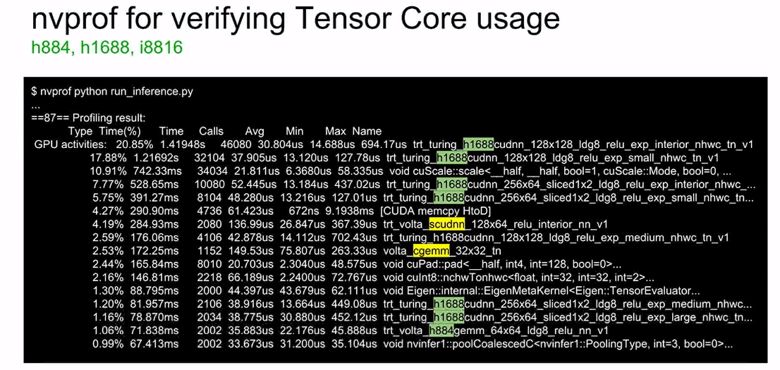
|
| Fig 9 Output of nvprof in the command prompt showing top kernels by compute time |
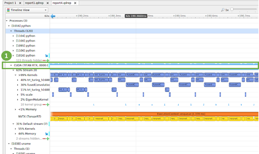
|
| Fig 10 NSIGHT Systems showing timeline view of a program utilizing the GPU well without major gaps |
Figure 10 highlights the timeline of CUDA kernels marked with (1). The goal here is to identify the largest gaps in the timeline, which indicates that the GPU is not performing computations at that time. The GPU would be either waiting for data to be available or for a CPU operation to complete. Since ResNet-50 is well optimized, you notice that the gaps between kernels is very small of the order of few microseconds. If your graph has larger gaps, this is a lead to investigate what operations cause the gaps. You can also see in the image above the CUDA streams and their corresponding CUDA kernels. The yellow corresponds to TensorRT layers. An exhaustive treatment of debugging workflows is outside the scope of this blog.
You can see in figure 11 that a gap in the compute timeline corresponding to when the GPU is not utilized. You want to investigate patterns like this further.
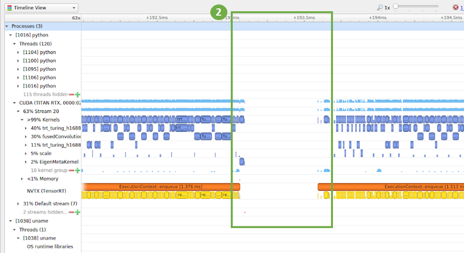
|
| Fig 11 NSIGHT Systems showing the timeline view for a program that has gap in GPU utilization |
Vision and NLP represent common use cases requiring these tools for processing application input. If pre-processing of these applications is slow because of unavailability of data or network bottlenecks, using the tools above will help you identify areas to optimize your application. We often see that the bottleneck in the pipeline for inference in TF-TRT is loading inputs from disks or networks (such as jpeg images or TFRecords) and preprocessing them before feeding them into the inference engine. If data pre-processing is a bottleneck, you should explore using I/O libraries such as
nvidia/dali to accelerate them using optimizations such as multithreaded I/O and image processing and performing image processing on GPUs.
TensorFlow Profiler is another tool that ships with TensorFlow and is handy for visualizing kernel timing information by putting additional parameters in the Python script. Examples include additional
options and
run_metadata provided to the session run:
sess.run(res, options=options, run_metadata=run_metadata). After execution, a .json file with profiled data is generated in Chrome trace format and can be viewed by the Chrome browser.
You can use the TensorFlow logging capability as well as TensorBoard to see what parts of your application are converted to TensorRT. To use logging, increase the verbosity level in TensorFlow logs to print logs from a selected set of C++ files. You can learn more about verbose logging and levels allowed in the
Debugging Tools documentation. See example code to increase verbosity level below:
TF_CPP_VMODULE=segment=2,convert_graph=2,convert_nodes=2,trt_engine_op=2 python run_inference.py
The other option is to visualize the graph in
TensorBoard, a suite of visualization tools for TensorFlow. TensorBoard allows you to examine the TensorFlow graph, what nodes are in it, what TensorFlow nodes are converted to TensorRT node, what nodes are attached to TensorRT nodes, and even the shape of the tensors in the graph. Learn more in
Visualizing TF-TRT Graphs With TensorBoard.
Is your algorithm using Tensor Cores?
You can use
nvprof to check if your algorithm is using Tensor Cores. Figure 9 above shows an example of measuring performance using
nvprof with the inference python script:
nvprof python run_inference.py When using Tensor Cores with FP16 accumulation, the string ‘h884’ appears in the kernel name. On Turing, kernels using Tensor Cores may have ‘s1688’ and ‘h1688’ in their names, representing FP32 and FP16 accumulation respectively.
If your algorithm is not using Tensor Cores, you can do a few things to debug and understand why. In order to check if Tensor Cores are used for my network, follow these steps:
- Use command
nvidia-smi on the command line to confirm that the current hardware architecture are Volta or Turing GPUs.
- Operators such as Fully Connected, MatMul, and Conv can use Tensor Cores. Make sure that all dimensions in these ops are multiples of 8 to trigger Tensor Core usage. For Matrix multiplication: M, N, K sizes must be multiples of 8. Fully-connected layers should use multiple-of-8 dimensions. If possible, pad input/output dictionaries to multiples of 8.
Note that in some cases TensorRT might select alternative algorithms not based on Tensor Cores if they perform faster for the chosen data and operations. You can always report bugs and interact with the TensorFlow-TensorRT community in the
TensorRT forum.
Performance and Benchmarking Scripts
TensorRT maximizes inference performance, speeds up inference, and delivers low latency across a variety of networks for image classification, object detection, and segmentation. ResNet-50, as an example, achieves up to 8x higher throughput on GPUs using TensorRT in TensorFlow. You can achieve high throughput while maintaining high accuracy due to support of INT8 quantization. Find the latest performance results on NVIDIA GPU platforms in the
Deep Learning Product Performance page.
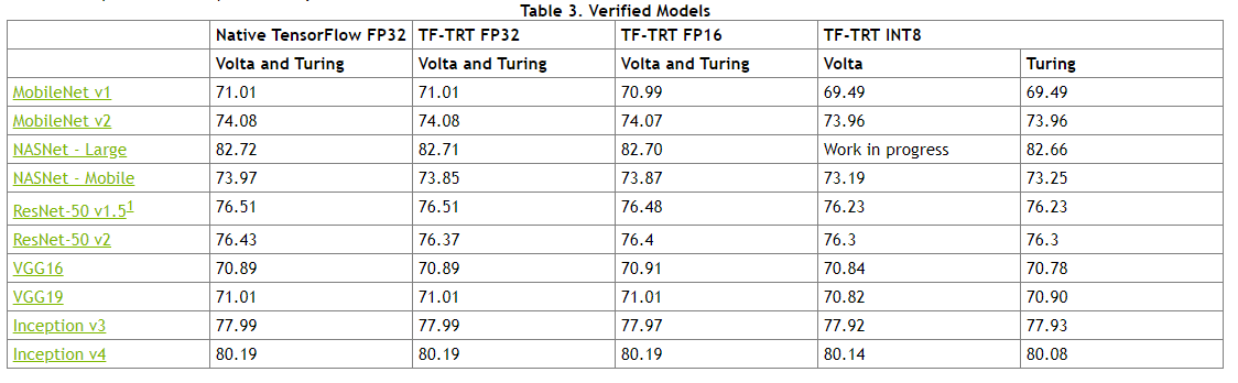
Table 1 below shows accuracy numbers for each model that we validate against in our March 2019 containers. Our validation runs inference on the whole ImageNet validation dataset and provides the top-1 accuracy. Find the set of benchmarked models and accuracy numbers in the
verified models section of the TensorFlow-TensorRT documentation.
|
| Table 1: Accuracy numbers for common models from the documentation for 19.03 containers |
You can use our scripts in the
tensorflow/tensorrt github repo to download and benchmark these models, which uses publicly available models (ResNet, MobileNet, Inception, VGG, NASNet L/M, SSD MobileNet v1) from
TF slim and
TF official.
What’s Next
TensorFlow 2.0 was announced at the TensorFlow Developer Summit in April 2019 and is available in alpha at the time of writing this blog. TensorRT has been moved to the core compiler repository from the contrib area. The APIs have changed slightly, but older APIs will continue to be supported. See the updated code snippet to apply TensorRT optimizations to the TensorFlow graph in TensorFlow 2.0:
from tensorflow.python.compiler.tensorrt import trt_convert as tru
params = trt.DEFAULT_TRT_CONVERSION_PARAMS._replace(
    precision_mode='FP16')
converter = trt.TrtGraphConverterV2(
input_saved_model_dir=input_saved_model_dir, conversion_params=params)
converter.convert()
converter.save(output_saved_model_dir)
TensorFlow 1.14, which is expected shortly, would use the
TrtGraphConverter function with the remaining code staying the same.
Over to You
We expect the TensorFlow-TensorFlowRT integration to ensure the highest performance possible when using NVIDIA GPUs while maintaining the ease and flexibility of TensorFlow. Developers will automatically benefit from updates as TensorRT supports more networks, without any changes to existing code.
This article is based on a talk at the GPU Technology Conference, 2019 in San Jose. See the full length recording of the “
TensorRT inference With TensorFlow” talk to learn more.
The integration will also be available in the
NVIDIA GPU Cloud (NGC) TensorFlow container. We believe you’ll see substantial benefits to integrating TensorRT with TensorFlow when using GPUs for inference. The
TensorRT page offers more information on TensorRT as well as links to further articles and documentation.
NVIDIA strives to constantly improve its technologies and products, so please let us know what you think by leaving a comment below.


