Posted by Gábor Bartók and Efi Kokiopoulou, Google Research
This article assumes you have some prior experience with reinforcement learning and/or multi-armed bandits. If you’re new to the subject, a good starting point is the Bandits Wikipedia entry, or for a bit more technical and in-depth introduction, this book.
In this blog post we introduce the TensorFlow-Agents Bandits library. This library offers a comprehensive list of the most popular bandit algorithms along with a variety of test problems on which the algorithms can be run. The test problems (called bandit environments) include some synthetic environments as well as environments converted from real-life (classification or recommendation) datasets.
One of the latter is the MovieLens environment, which utilizes this dataset. In this blog post, we will guide you through the usage of the TF-Agents Bandits library with the help of the MovieLens Environment.
Multi-Armed Bandits is a machine learning framework in which an agent repeatedly selects actions from a set of actions and collects rewards by interacting with the environment. The goal of the agent is to accumulate as much reward as possible, within a given time horizon. The name “bandit” comes from the illustrative example of finding the best slot machine (one-armed bandit) from a set of machines with different payoffs. The actions are also known as “arms”.
 |
| Image from Wikipedia |
There are two more important concepts to be aware of: “context”, and “regret”. In many real life scenarios, it’s not enough to find the best action that on average provides the highest reward: we want to find the best action depending on the situation/context. To extend the bandits framework in this direction, we introduce the notion of “context”. Before the agent has to select an action, it receives the context that provides information about the current round. Then the agent’s goal is to find the policy that selects the highest-rewarding action for the given context.
In bandits literature, the notion of “regret” is very important. The regret can be informally defined as the difference in performance between the optimal policy and the learned policy. Typically the performance is measured in terms of cumulative reward (i.e., sum of rewards across several rounds); otherwise, one may also refer to the “instantaneous regret” which is the regret the agent suffers at a certain round. Bandit algorithms typically come with performance guarantees in terms of upper bound on the regret given a family of bandit problems.
Consider the following scenario. You are tasked with recommending movies to users of a movie streaming service. In every round you receive information about the user. Your task is to choose from a handful of movies for the user with the goal of choosing one that the user will enjoy and give a high rating.
For illustration purposes, we will turn the well-known MovieLens dataset into a bandit problem. The dataset consists of ~100K ratings from 943 users on 1682 movies. Our first step to turn this dataset into a contextual bandit problem is to construct the matrix `A` of user/movie ratings, where `A_ij` is the rating of user `i` of movie `j`. Since we have the ratings to a few movies only from each user, one issue with the ratings matrix `A` is that it is very sparse i.e., only a few entries `A_ij` are available; all the other entries are unknown. To address this sparsity issue, we construct a low-rank SVD decomposition `A ~= U*V’` (low-rank matrix decomposition in recommender systems is a popular approach for collaborative filtering, see e.g., Koren et al. 2009). This way, the rows of `U` are context features. Then, the movies to be recommended to the user are the set of actions, represented as rows of `V`. The reward for recommending movie `j` to user `i` can then be calculated as the inner product of the corresponding rows of `U_i` and `V_j`. Therefore, using the low-rank SVD decomposition to compute rewards gives us the ability to approximate the reward even for movies that were not recommended to the users; hence their rating was unknown.
Now let’s see how the above problem is modeled and solved with the help of the TF-Agents Bandits library. TF-Agents is a modular library that has building blocks for every aspect of Reinforcement Learning and Bandits. A problem can be expressed in terms of an “environment”. An environment is a class that generates observations (aka contexts), and also outputs a reward after being presented with actions. In the case of the MovieLens environment, an observation is a random row of the matrix `U`, while the reward is given after an algorithm has chosen an action (i.e., row of the matrix `V`, a movie in our case). The implementation of the MovieLens environment can be found here. It’s worth noting here that it is rather simple to implement a bandit environment in TF-Agents. For a walkthrough, we refer the reader to our Bandits Tutorial.
Bandit algorithms in TF-Agents have two main building blocks: “policies” and “agents”. A policy is a function that, given an observation, chooses an action. The agent is responsible for learning a good policy: given examples of (observation, action, reward) tuples, it trains the policy so that it chooses better actions. The TF-Agents Bandits library offers a comprehensive list of the most popular algorithms, including linear methods as well as nonlinear ones (e.g., those with neural network-based value functions). Let’s see how LinUCB tackles the MovieLens problem!
In short, the LinUCB algorithm keeps track of running average rewards for all actions, along with confidence intervals around the estimates. In every turn, the algorithm chooses the action that has the highest upper confidence bound on its reward estimate.
In the TF-Agents library, the LinUCB algorithm is built from a LinearBanditPolicy with an “Optimistic Exploration Strategy”, and a LinearBanditAgent responsible for updating the estimates. Note that the exploration strategy can be changed from “Optimistic” to “Sampling”, in which case the algorithm becomes Linear Thompson Sampling.
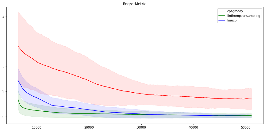
So let’s see how LinUCB performs on the MovieLens environment! We ran LinUCB on the MovieLens environment (with 100 actions and SVD decomposition rank 20) and we get results on TensorBoard:
(Note that all of the below plots are based on averaging five runs, the shadows show standard deviations. A rolling average smoothing is also applied on the curves.)

As mentioned above, with a slight modification of LinUCB, we get an implementation for Linear Thompson Sampling (LinTS). If we run LinTS on the same problem (implementation here), we get a very similar result to that of LinUCB (see joint graph further down).
Let’s compare these results with another agent, say, the NeuralEpsilonGreedy agent. As the name suggests, this agent uses a neural network to estimate the rewards, and adds uniform exploration with probability `epsilon`. This exploration strategy is known as “epsilon-greedy” since the method is greedy most of the time but with probability `epsilon` it explores by picking an action uniformly at random. If we run Neural Epsilon Greedy and put the results from the three algorithms, we get:
It’s interesting to also look at how often the methods pick suboptimal actions. This is shown below:
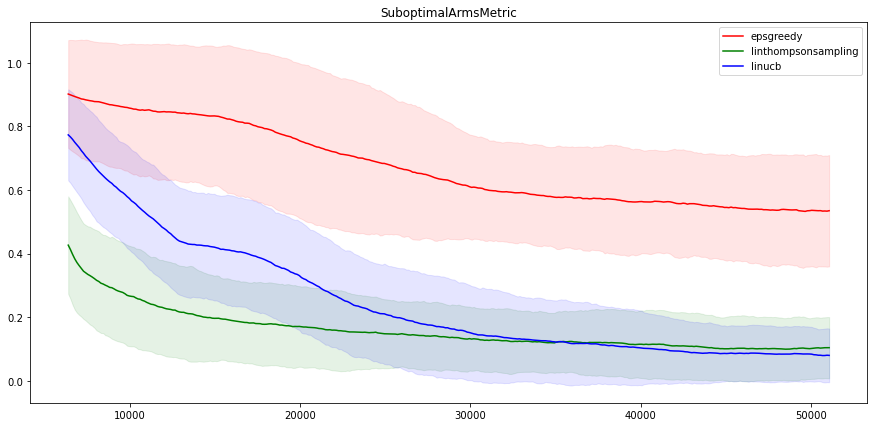
We see that LinUCB and LinTS have very similar performance, which is not very surprising, as they are very similar algorithms. On the other hand, Neural epsilon-Greedy is not doing very well on this problem. After fifty thousand iterations, the metrics are still far away from that of the linear methods. Note, nevertheless, that even the epsilon-Greedy algorithm manages to find the best movie about half the time, out of 100, still not bad!
To be fair, it’s expected that linear algorithms do better than non-linear ones on this problem, as the problem is linear (by the reward calculation construction).
As for the difference between the two linear algorithms, it seems that LinUCB struggles in the beginning a little bit, but in the long run it is slightly (not significantly) better than LinTS.
The MovieLens example above has some shortcomings: its actions are a selection of movies, algorithms have to learn a distinct model for every movie, and it’s also hard to introduce new movies in the system. To this end, we change the environment a little bit: instead of treating every movie as an independent action, we model the movies with features, similarly to users: the rows of `V` will be the movie features. Then the model only has to learn one reward function, whose input is both the user features `u` and the movie features `v`. This way we can have an unlimited number of movies in the system, and we can introduce new movies on the fly. This version of the environment can be found here.
Most of the agents implemented in our library have the functionality of running on environments that have features for its actions (we call these environments “per-arm environments”).
Now let’s see how the different algorithms behave on the per-arm version of the MovieLens environment. We ran the arm-feature versions of the three algorithms: LinUCB, LinTS, and eps-Greedy. The result is quite different from the previous section: Here the linear methods seem to fail to find the relationship between actions and rewards, while the neural approach gives similar results to that of the non-arm feature problem.
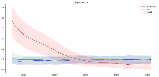
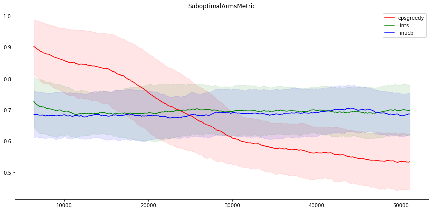
The neural algorithm still finds the best action ~45% of the time, while the linear algorithms only ~30% of the time.
If you haven’t found what you are looking for in the list of agents within the library, it’s possible, and not too complicated, to implement your own algorithm. You need to:
tf_agents.policies.TFPolicy and
tf_agents.agents.TFAgent.
To define a policy, one needs to implement its private member function _distribution(...). In short, this function takes an observation and outputs a distribution of actions (or simply an action in case of a deterministic policy).
As stated above, an agent is responsible for training the policy. To this end, subclasses of TF-Agents’ TFAgent (sorry) have to implement the private member function _train() (among others, some details are omitted for clarity). This function takes batches of training data, and trains the policy.
If you want to test your (new) algorithm and have an idea for an environment, it’s also simple to implement it in TF-Agents. A Bandit environment has two main roles: (i) to generate observations, and (ii) to return a reward after the agent chooses an action. One can easily create an environment class by defining these two functions.
In this blog post, we introduced the TF-Agents Bandit library and showed how to tackle a recommendation problem with it. If you want to play around with the environments and agents used in this post, you can go directly to this executable to run these agents and more. If you want to explore the library or just want to read more about it, we suggest starting with this tutorial. And if you’re interested in learning more about making recommendations on this MovieLens dataset, you can also check out another great library called TensorFlow Recommenders.
The TF-Agents Bandits library has been built in collaboration with Jesse Berent, Tzu-Kuo Huang, Kishavan Bhola, Sergio Guadarrama, Anoop Korattikara, Oscar Ramirez, Eugene Brevdo, and many others from the TF-Agents team.

July 22, 2021 — Posted by Gábor Bartók and Efi Kokiopoulou, Google Research This article assumes you have some prior experience with reinforcement learning and/or multi-armed bandits. If you’re new to the subject, a good starting point is the Bandits Wikipedia entry, or for a bit more technical and in-depth introduction, this book. In this blog post we introduce the TensorFlow-AgentsBandits library. This librar…


