Posted by Matthew Watson, Keras Developer
Determining the right feature representation for your data can be one of the trickiest parts of building a model. Imagine you are working with categorical input features such as names of colors. You could one-hot encode the feature so each color gets a 1 in a specific index ('red' = [0, 0, 1, 0, 0]), or you could embed the feature so each color maps to a unique trainable vector ('red' = [0.1, 0.2, 0.5, -0.2]). Larger category spaces might do better with an embedding, and smaller spaces as a one-hot encoding, but the answer is not clear cut. It will require experimentation on your specific dataset.
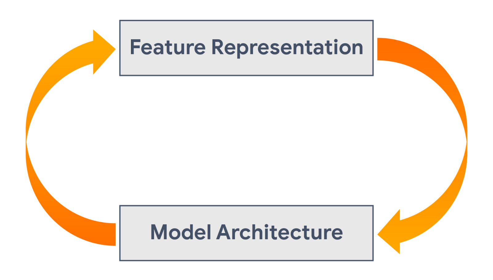
Ideally, we would like updates to our feature representation and updates to our model architecture to happen in a tight iterative loop, applying new transformations to our data while changing our model architecture. In practice, feature preprocessing and model building are usually handled by entirely different libraries, frameworks, or languages. This can slow the process of experimentation.
On the Keras team, we recently released Keras Preprocessing Layers, a set of Keras layers aimed at making preprocessing data fit more naturally into model development workflows. In this post we are going to use the layers to build a simple sentiment classification model with the imdb movie review dataset. The goal will be to show how preprocessing can be flexibly developed and applied. To start, we can import tensorflow and download the training data.
import tensorflow as tf
import tensorflow_datasets as tfds

train_ds = tfds.load('imdb_reviews', split='train', as_supervised=True).batch(32)
Keras preprocessing layers can handle a wide range of input, including structured data, images, and text. In this case, we will be working with raw text, so we will use the TextVectorization layer.
By default, the TextVectorization layer will process text in three phases:
A simple approach we can try here is a multi-hot encoding, where we only consider the presence or absence of terms in the review. For example, say a layer vocabulary is ['movie', 'good', 'bad'], and a review read 'This movie was bad.'. We would encode this as [1, 0, 1], where movie (the first vocab term) and bad (the last vocab term) are present.
text_vectorizer = tf.keras.layers.TextVectorization(
     output_mode='multi_hot', max_tokens=2500)
features = train_ds.map(lambda x, y: x)
text_vectorizer.adapt(features)
Above, we create a TextVectorization layer with multi-hot output, and do two things to set the layer’s state. First, we map over our training dataset and discard the integer label indicating a positive or negative review. This gives us a dataset containing only the review text. Next, we adapt() the layer over this dataset, which causes the layer to learn a vocabulary of the most frequent terms in all documents, capped at a max of 2500.
Adapt is a utility function on all stateful preprocessing layers, which allows layers to set their internal state from input data. Calling adapt is always optional. For TextVectorization, we could instead supply a precomputed vocabulary on layer construction, and skip the adapt step.
We can now train a simple linear model on top of this multi-hot encoding. We will define two functions: preprocess, which converts raw input data to the representation we want for our model, and forward_pass, which applies the trainable layers.
def preprocess(x):
  return text_vectorizer(x)

def forward_pass(x):
  return tf.keras.layers.Dense(1)(x)  # Linear model

inputs = tf.keras.Input(shape=(1,), dtype='string')
outputs = forward_pass(preprocess(inputs))
model = tf.keras.Model(inputs, outputs)
model.compile(loss=tf.keras.losses.BinaryCrossentropy(from_logits=True))
model.fit(train_ds, epochs=5)
That’s it for an end-to-end training example, and already enough for 85% accuracy. You can find complete code for this example at the bottom of this post.
Let’s experiment with a new feature. Our multi-hot encoding does not contain any notion of review length, so we can try adding a feature for normalized string length. Preprocessing layers can be mixed with TensorFlow ops and custom layers as desired. Here we can combine the tf.strings.length function with the Normalization layer, which will scale the input to have 0 mean and 1 variance. We have only updated code up to the preprocess function below, but we will show the rest of training for clarity.
# This layer will scale our review length feature to mean 0 variance 1.
normalizer = tf.keras.layers.Normalization(axis=None)
normalizer.adapt(features.map(lambda x: tf.strings.length(x)))

def preprocess(x):
  multi_hot_terms = text_vectorizer(x)
  normalized_length = normalizer(tf.strings.length(x))
  # Combine the multi-hot encoding with review length.
  return tf.keras.layers.concatenate((multi_hot_terms, normalized_length))

def forward_pass(x):
  return tf.keras.layers.Dense(1)(x)  # Linear model.

inputs = tf.keras.Input(shape=(1,), dtype='string')
outputs = forward_pass(preprocess(inputs))
model = tf.keras.Model(inputs, outputs)
model.compile(loss=tf.keras.losses.BinaryCrossentropy(from_logits=True))
model.fit(train_ds, epochs=5)
Above, we create the normalization layer and adapt it to our input. Within the preprocess function, we simply concatenate our multi-hot encoding and length features together. We learn a linear model over the union of the two feature representations.
The last change we can make is to speed up training. We have one major opportunity to improve our training throughput. Right now, every training step, we spend some time on the CPU performing string operations (which cannot run on an accelerator), followed by calculating a loss function and gradients on a GPU.
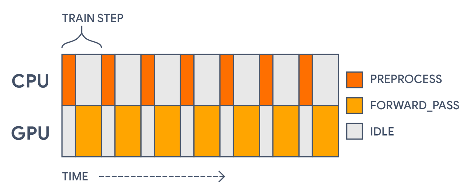 |
| With all computation in a single model, we will first preprocess each batch on the CPU and then update parameter weights on the GPU. This leaves gaps in our GPU usage. |
This gap in accelerator usage is totally unnecessary! Preprocessing is distinct from the actual forward pass of our model. The preprocessing doesn't use any of the parameters being trained. It’s a static transformation that we could precompute.
To speed things up, we would like to prefetch our preprocessed batches, so that each time we are training on one batch we are preprocessing the next. This is easy to do with the tf.data library, which was built for uses like this. The only major change we need to make is to split our monolithic keras.Model into two: one for preprocessing and one for training. This is easy with Keras’ functional API.
inputs = tf.keras.Input(shape=(1,), dtype="string")
preprocessed_inputs = preprocess(inputs)
outputs = forward_pass(preprocessed_inputs)

# The first model will only apply preprocessing.
preprocessing_model = tf.keras.Model(inputs, preprocessed_inputs)
# The second model will only apply the forward pass.
training_model = tf.keras.Model(preprocessed_inputs, outputs)
training_model.compile(
    loss=tf.keras.losses.BinaryCrossentropy(from_logits=True))

# Apply preprocessing asynchronously with tf.data.
# It is important to call prefetch and remember the AUTOTUNE options.
preprocessed_ds = train_ds.map(
    lambda x, y: (preprocessing_model(x), y),
    num_parallel_calls=tf.data.AUTOTUNE).prefetch(tf.data.AUTOTUNE)

# Now the GPU can focus on the training part of the model.
training_model.fit(preprocessed_ds, epochs=5)
In the above example, we pass a single keras.Input through our preprocess and forward_pass functions, but define two separate models over the transformed inputs. This slices our single graph of operations into two. Another valid option would be to only make a training model, and call the preprocess function directly when we map over our dataset. In this case, the keras.Input would need to reflect the type and shape of the preprocessed features rather than the raw strings.
Using tf.data to prefetch batches cuts our train step time by over 30%! Our compute time now looks more like the following:
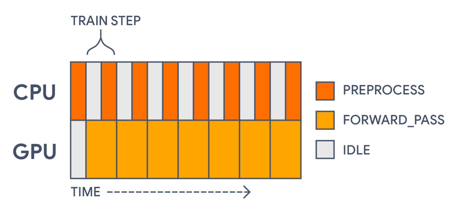 |
| With tf.data, we are now precomputing each preprocessed batch before the GPU needs it. This significantly speeds up training. |
We could even go a step further than this, and use tf.data to cache our preprocessed dataset in memory or on disk. We would simply add a .cache() call directly before the call to prefetch. In this way, we could entirely skip computing our preprocessing batches after the first epoch of training.
After training, we can rejoin our split model into a single model during inference. This allows us to save a model that can directly handle raw input data.
inputs = preprocessing_model.input
outputs = training_model(preprocessing_model(inputs))
inference_model = tf.keras.Model(inputs, outputs)
inference_model.predict(
    tf.constant(["Terrible, no good, trash.", "I loved this movie!"]))
Keras preprocessing layers aim to provide a flexible and expressive way to build data preprocessing pipelines. Prebuilt layers can be mixed and matched with custom layers and other tensorflow functions. Preprocessing can be split from training and applied efficiently with tf.data, and joined later for inference. We hope they allow for more natural and efficient iterations on feature representation in your models.
To play around with the code from this post in a Colab, you can follow this link. To see a wide range of tasks you can do with preprocessing layers, see the Quick Recipes section of our preprocessing guide. You can also check out our complete tutorials for basic text classification, image data augmentation, and structured data classification.

noviembre 24, 2021 — Posted by Matthew Watson, Keras Developer Determining the right feature representation for your data can be one of the trickiest parts of building a model. Imagine you are working with categorical input features such as names of colors. You could one-hot encode the feature so each color gets a 1 in a specific index ('red' = [0, 0, 1, 0, 0]), or you could embed the feature so each color ma…


