desember 01, 2021 — A guest post by Chansung Park, Sayak Paul (ML-GDEs) Continuous integration and delivery (CI/CD) is a much sought-after topic in the DevOps domain. In the MLOps (Machine Learning + Operations) domain, we have another form of continuity -- continuous evaluation and retraining. MLOps systems evolve according to the changes of the world, and that is usually caused by data/concept drift. So, to cater …

A guest post by Chansung Park, Sayak Paul (ML-GDEs)
Continuous integration and delivery (CI/CD) is a much sought-after topic in the DevOps domain. In the MLOps (Machine Learning + Operations) domain, we have another form of continuity -- continuous evaluation and retraining. MLOps systems evolve according to the changes of the world, and that is usually caused by data/concept drift. So, to cater to the data changes we need to continuously evaluate our deployed ML models and retrain and re-deploy them as necessary.
In this blog post, we present a project that implements a workflow combining batch prediction and model evaluation for continuous evaluation retraining In order to capture changes in the data. We will first discuss the general setup of the project. Then we will move on to key components (batch prediction, new data spans, retraining, etc.) that are important for continuously evaluating an ML model and then re-training it if needed. Rather than discussing the technical implementation details of the project, we will keep it high-level so that we will focus on understanding the underlying concepts.
The project is implemented with TensorFlow Extended (TFX), Keras, and various services offered from Google Cloud Platform. You can find the project on GitHub.
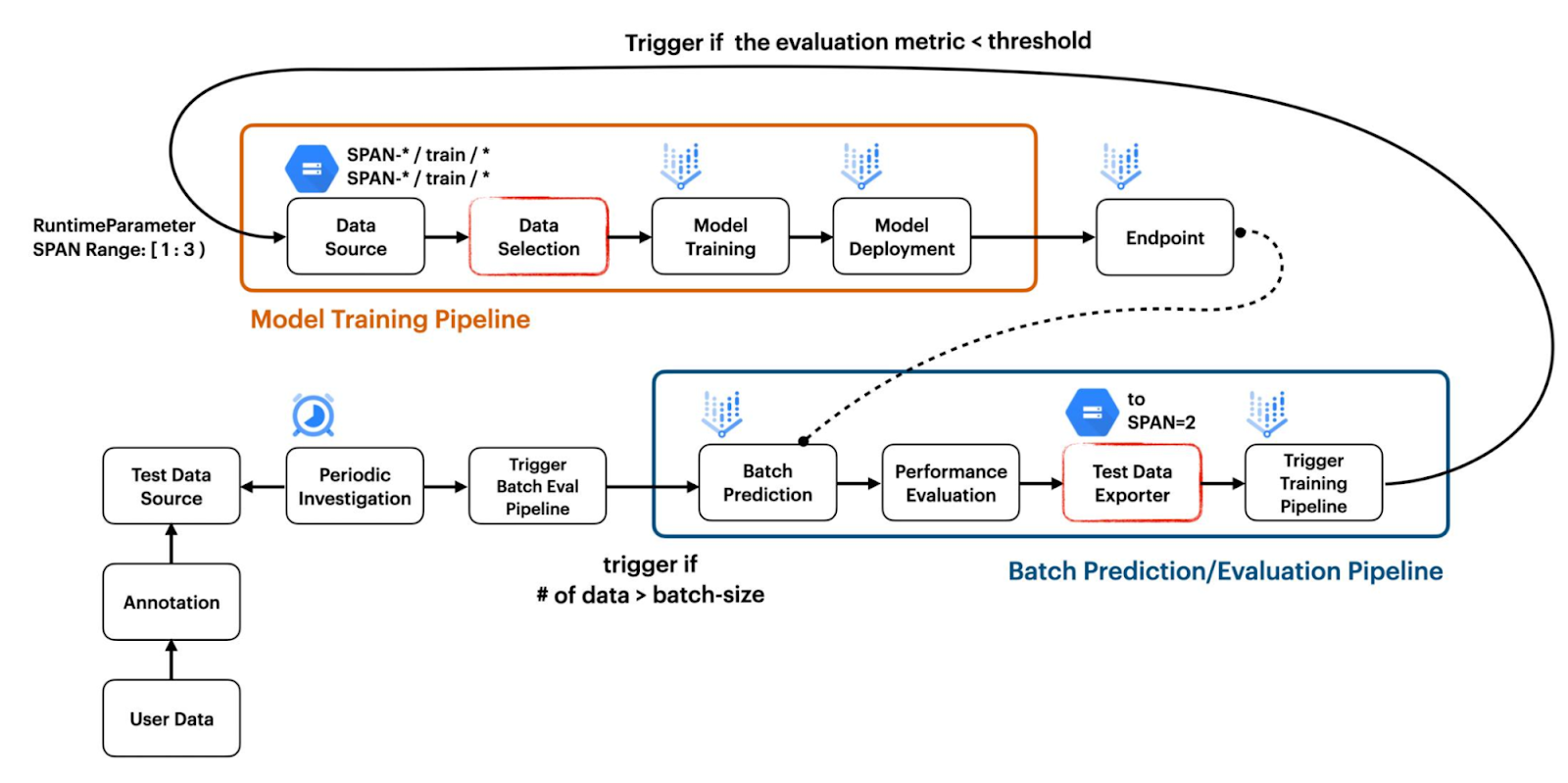
This project shows how to build two separate pipelines working together to create a CI/CD workflow which responds to changes in the data. The first pipeline is for model training, and the second pipeline is for model evaluation based on the result of a batch prediction as shown in Figure 1.
 |
| Figure 1. Overview of the project structure (original) |
The model training pipeline is built by combining standard TFX components such as ImportExampleGen and Trainer with custom TFX components such as VertexUploader and VertexDeployer. Since the Pusher standard component had an issue when we were doing this project, we have brought custom components from our previous project, Dual Deployments.
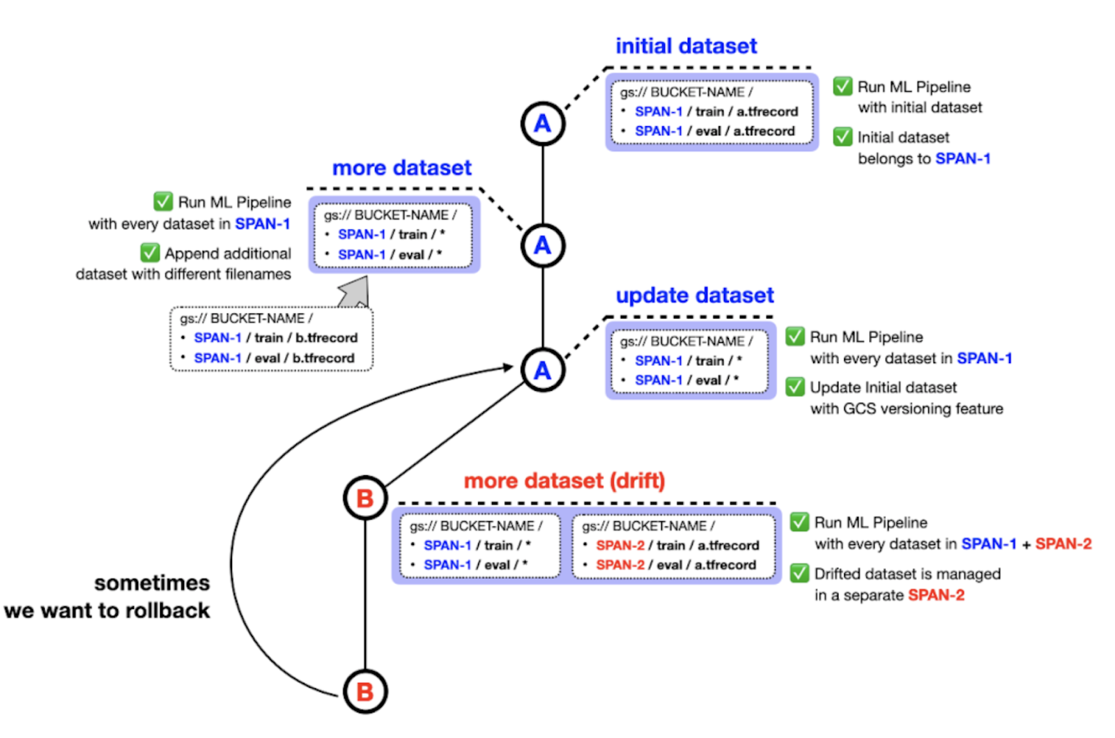
There is one significant implementation detail on how ImportExampleGen handles the dataset to be fed into the model. We have designed our project to hold datasets from different distributions in separate folders with filesystem paths which indicate the span number. For instance, the initial training and test dataset can be stored in SPAN-1/train and SPAN-2/test while the drifted dataset can be stored in SPAN-2/train and SPAN-2/test respectively as shown in Figure 2.
For the sake of the versioning feature in Google Cloud Storage (GCS), you might think we don’t need to manage datasets in this manner. However, we thought our way makes datasets much more manageable. For example, you might want to pick data from SPAN-1 and SPAN-2 or SPAN-1 and SPAN-3 to train the model depending on situations. Also, datasets belonging to the same distribution can still benefit from the versioning feature in GCS.
 |
| Figure 2. How datasets are managed (original) |
The batch evaluation pipeline does not leverage any standard TFX components. Rather it consists of five custom TFX components which are FileListGen, BatchPredictionGen, PerformanceEvaluator, SpanPreparator, and PipelineTrigger. These components are available as standalone modules here.
 |
| Figure 3. Custom TFX components in batch evaluation pipeline (original) |
FileListGen generates a text file to be looked up by the currently deployed model on Vertex AI to perform batch prediction according to the format required by Vertex Prediction. Then BatchPredictionGen will simply perform Vertex Prediction based on the prepared text file from the FileListGen and output a set of files containing the batch prediction results. PerformanceEvaluator calculates the average accuracy based on the batch prediction results and outputs False if it is less than the threshold. If the output is True, the pipeline will be terminated. Or if the output is False, SpanPreparator prepares TFRecord files by compressing the list of raw data, and then puts those TFRecords into a new folder whose name contains the successive span number such as span-2. Finally, PipelineTrigger triggers the model training pipeline by passing the span numbers for the data which should be included for training the model through RuntimeParameter.
In this section, we walk through the key components of the project and also leave some notes on the tools we used to implement them.
We focus on the concepts and consider implementing them in a minimal manner so that our implementations are as reproducible and as accessible as possible. Keeping that in mind, we use the CIFAR-10 training set as our training data and we fine-tune a ResNet50 model to fit the data. Our training pipeline is demonstrated in this notebook.
To simulate a data drift scenario, we then collect a bunch of images from the internet matching CIFAR-10 classes. To make it easy to follow we implement this workflow inside a Colab Notebook which is available here. This workflow also includes uploading and deploying the trained model as a service on the Vertex AI platform.
We then perform inference on these images with the trained model from the above step. We perform batch inference rather than online inference to get the results. We use Vertex AI’s batch prediction service to realize this. In practice, usually after this step, the model test images and model predictions are sent to domain experts for audit purposes. They also provide the expected ground-truth labels on the test images. Only after that, we can validate the prediction results. But for the purpose of this project, we eliminate this step and pretend that the ground-truth labels are already available. So, as soon as the batch prediction results are available we evaluate them. This entire workflow is covered in this notebook.
We deploy a Cloud Function to monitor a specific location inside a Google Cloud Storage (GCS) bucket. If there is a sufficient number of new test images available inside that location, we trigger the batch prediction pipeline. We cover this workflow in this notebook. This is how we achieve the “continuous evaluation” aspect of our project.
There are other ways to capture drift in data, though. For example, using JS-Divergence, we can compare the distributions between the newly available data and training data. You can follow this Coursera lecture from Robert Crowe which dives deep into these techniques.
After the batch predictions are evaluated, the next step is to determine if we need to re-train the model based on a predefined performance threshold that generally depends on the business context and a lot of other factors. We set this threshold to 0.9 in the project. If we need to re-train then we trigger the same model training pipeline (as shown in this notebook) but with the newly available data added to the CIFAR-10 training set. We can either warm-start our model from a previous checkpoint or we can train the model from scratch using all the available training data. For this project, we do the latter.
In the following section, we will go over a few non-trivial components from our implementation and discuss their motivation and technicalities. As a reminder, our implementation is fully open-sourced here.
In this section, we walk through the implementation details on some key aspects of the project. Please go through the project repository and review all notebooks for further information.
The initial CIFAR-10 datasets are stored in {bucket-name}/span-1/train and {bucket-name}/span-1/test GCS locations respectively. This step is done through the first notebook. Then, we download more images of the same categories as in CIFAR-10 by using Bing Image Downloader. Those images are resized by 32x32 to make them compatible with CIFAR-10 datasets, and they are stored in a separate GCS bucket such as {bucket-batch-prediction}/2021-10/.
Note we used the YYYY-MM for the name where the images are stored. This is because Cloud Function which is fired by Cloud Scheduler will look for the latest GCS location to launch the batch evaluation pipeline as shown below.
def get_latest_directory(storage_client, bucket):
    blobs = storage_client.list_blobs(bucket)

    folders = list(
        set(
            [
                os.path.dirname(blob.name)
                for blob in blobs
                if bool(
                    re.match(
                        "[1-9][0-9][0-9][0-9]-[0-1][0-9]", os.path.dirname(blob.name)
                    )
                )
                is True
            ]
        )
    )

    folders.sort(key=lambda date: datetime.strptime(date, "%Y-%m"))
    return folders[0]
As you see, it only looks for the GCS location that exactly matches the YYYY-MM format. The Cloud Function launches the batch evaluation pipeline by passing which GCS location to look up for batch prediction via RuntimeParameter. The code snippet below shows how it is passed to the pipeline with the name data_gcs_prefix on the Cloud Function side.
from kfp.v2.google.client import AIPlatformClient

api_client = AIPlatformClient(project_id=project, region=region)

response = api_client.create_run_from_job_spec(
     ...
     parameter_values={"data_gcs_prefix": latest_directory},
)
The pipeline recognizes data_gcs_prefix is a type of RuntimeParameter, and it is used in the FileListGen component which prepares a text file in the required format to perform Vertex AI Batch Prediction.
def _create_pipeline(
    data_gcs_prefix: data_types.RuntimeParameter,
    ...
) -> Pipeline:

   filelist_gen = FileListGen(
        ...
        gcs_source_bucket=data_gcs_bucket,
        gcs_source_prefix=data_gcs_prefix,
    ).with_id("filelist_gen")

    ....
Let’s skip the batch prediction performed by the BatchPredictionGen component.
When the PerformanceEvaluator component determines that retraining should be performed based on the result from the BatchPredictionGen component, the SpanPreparator prepares a TFRecord file with the newly collected images, moves it to {bucket-name}/span-1/train and {bucket-name}/span-2/test where the training pipeline is ingesting data for model training, and renames the GCS location where the newly collected images are to {bucket-batch-prediction}/YYYY-MM_old/.
We add the _old suffix so that Cloud Function will ignore the renamed GCS location. If the retrained model doesn’t show a good enough performance metric, then you can have a chance to collect more data and merge them with the images in the _old GCS location.
The PipelineTrigger component at the end of the batch evaluation pipeline will trigger the training pipeline by passing which span numbers to look for in order to do model training. The data will be consumed by ImportExampleGen, based on the glob pattern matching feature. For instance, if data from span-1 and span-2 should be used for model training, then the glob pattern for the training dataset might be span-[12]/train/*.tfrecord. The code snippet below clearly shows the generalized version of the idea.
response = api_client.create_run_from_job_spec(
 ...
 parameter_values={
  "input-config": json.dumps(
      {
         "splits": [
             {
                "name": "train",
                "pattern": f"span-[{int(latest_span)-1}{latest_span}]/train/*.tfrecord",
             },
             {
                "name": "val",
                "pattern": f"span-[{int(latest_span)-1}{latest_span}]/test/*.tfrecord",
             },
        ]
      }
  ),
  "output-config": json.dumps({}),
 },
)
The reason we formed the RuntimeParameter in the parameter_values in this way is that the pattern matching feature of the ImportExampleGen component should be specified in the input-config and output-config parameters. We do not need the output-config parameter for our purpose, but it is required when passing the input-config parameter as a RuntimeParameter. That’s why the output-config parameter is left empty. Note that you have to form the parameter in protocol buffer format when using RuntimeParameter for standard TFX components. The code below shows how the passed input-config and output-config can be consumed by the ImportExampleGen component.
example_gen = tfx.components.ImportExampleGen(
     input_base=data_root, input_config=input_config, output_config=output_config
)
It is worth noting that you can leverage the rolling window feature supported by TFX with the standard components if the backend environment is Kubeflow Pipeline v1. The code snippet below shows how to achieve this with the CsvExampleGen component and a Resolver node.
examplegen_range_config = proto.RangeConfig(
     static_range=proto.StaticRange(
         start_span_number=2, end_span_number=2))

example_gen = tfx.components.CsvExampleGen(
     input_base=data_root,
     input_config=examplegen_input_config,
     range_config=examplegen_range_config)

resolver_range_config = proto.RangeConfig(
     rolling_range=proto.RollingRange(num_spans=2))

examples_resolver = tfx.dsl.Resolver(
     strategy_class=tfx.dsl.experimental.SpanRangeStrategy,
     config={
         'range_config': resolver_range_config
     },
     examples=tfx.dsl.Channel(
         type=tfx.types.standard_artifacts.Examples,
         producer_component_id=example_gen.id)).with_id('span_resolver')
This is a much better way since it reuses the artifacts generated by the previous ExampleGens, and the current pipeline run only takes care of the data in the new span. Unfortunately however this feature is not supported by Vertex AI Pipeline which is based on Kubeflow Pipeline v2. We had an extensive discussion with the TFX team about this, which is why we came up with a different approach from the standard way.
Vertex AI Training is a separate service from Pipeline. We need to pay for the Vertex AI Pipeline individually, and at the time of writing this article, it costs about $0.03 USD per pipeline run. The type of compute instance for each TFX component was e2-standard-4, and it costs about $0.134 per hour. Since the whole pipeline took less than an hour to be finished, we can estimate that the total cost was about $0.164 for a Vertex AI Pipeline run.
The cost of custom model training depends on the type of machine and the number of hours. Also, you have to consider that you pay for the server and the accelerator separately. For this project, we chose n1-standard-4 machine type whose price is $0.19 per hour and NVIDIA_TESLA_K80 accelerator type whose price is $0.45 per hour. The training for each model was done in less than an hour, so it cost about $1.28 in total. So, as per our estimates, the upper bound of the costs incurred should not be more than $5.
The cost only stems from Vertex AI because the rest of the components like Pub/Sub, Cloud Functions, etc., have very minimal usage. So even if we add a small estimate for those costs, the upper bound of the total cost for this project should not be more than $5. Please refer to the official documents on the price: Vertex AI price reference, Cloud Build price reference.
In any case, you should use this GCP Price Calculator to get a better understanding of how your cost for the GCP services might differ.
In this blog post, we touched upon the idea of continuous evaluation and re-training for machine learning systems as well as the tooling needed to implement them. There is also a more traditional form of CI/CD for ML systems in response to code changes including changes in hyperparameters, model architecture, etc. We have a separate project demonstrating that use case. You are encouraged to check them here: Part I and Part II.
We are grateful to the ML-GDE program that provided GCP credits for supporting our experiments. We sincerely thank Robert Crowe and Jiayi Zhao of Google for their help with the review.

desember 01, 2021 — A guest post by Chansung Park, Sayak Paul (ML-GDEs) Continuous integration and delivery (CI/CD) is a much sought-after topic in the DevOps domain. In the MLOps (Machine Learning + Operations) domain, we have another form of continuity -- continuous evaluation and retraining. MLOps systems evolve according to the changes of the world, and that is usually caused by data/concept drift. So, to cater …