Posted by Nived P A, Margaret Maynard-Reid, Joel Shor
Google Summer of Code is a program that brings student developers into open-source projects each summer. This article describes enhancements made to the TensorFlow GAN library (TF-GAN) last summer that were proposed by Nived PA, an undergraduate student of Amrita School of Engineering. The goal of Nived’s project was to improve the TF-GAN library by adding new tutorials, and adding new functionality to the library itself.
This article provides an overview of TF-GAN and our accomplishments from last summer. We will share our experience from the perspective of both the student and the mentors, and walk through one of the new tutorials Nived created, an ESRGAN TensorFlow implementation, and show you how easy it is to use TF-GAN to help with training and evaluation.
TF-GAN provides common building blocks and infrastructure support for training GANs, and offers easy-to-use, standard techniques for evaluating them. Using TF-GAN helps developers and researchers save time with common GAN tools, and avoids common pitfalls in implementations. In addition, TF-GAN offers a collection of famous examples that include GANs from the image and audio space, as well as GPU and TPU support.
Since its launch in 2017, the team has updated the infrastructure to work with TensorFlow 2.0, released a self-study GAN course viewed by over 150K people in 2020, and an ML Tech talk on GANs. The project itself has been downloaded over millions of times. Papers using TF-GAN have thousands of citations (e.g. 1, 2, 3, 4, 5).
The TF-GAN library can be divided into a number of independent parts, namely Core, Features, Losses, Evaluation and Examples. Each of these different parts can be used to simplify the training or evaluation process of GANs.
The Google Summer of Code 2021 project on TF-GAN was aimed at adding more recent GAN models as examples to the library and additionally add more tutorial notebooks that explored various functionalities of TF-GAN while training and evaluating state-of-the-art GAN models such as ESRGAN. Through this project new loss functions were also added to the library that can improve the training process of GANs. Next, we will walk through the ESRGAN code and demonstrate how to use TF-GAN to help with training and evaluation.
If you are new to GANs, a good start is to read this Intro to GANs post written by Margaret (who mentored this project), these GANs tutorials on tensorflow.org and the self-study GAN course on Machine Learning Crash Course as mentioned above.
Image super resolution is an important use case of GANs. Super resolution is the process of reconstructing a high resolution (HR) image from a given low resolution (LR) image. Super resolution can be applied to solve real world problems such as photo editing.
The SRGAN paper (Photo-Realistic Single Image Super-Resolution Using a Generative Adversarial Network) introduced the concept of single-image super resolution and used residual blocks and perception loss to achieve that. The ESRGAN (Enhanced Super-Resolution Generative Adversarial Networks) paper enhanced SRGAN by introducing the Residual-in-Residual Dense Block (RRDB) without batch normalization as the basic building block, using relativistic loss and improved the perceptual loss.
Now let’s walk through how to implement ESRGAN with TensorFlow 2 and evaluate its performance with TF-GAN. There are two versions of Colab notebook: one using GPU and the other one using TPU. We will be going over the Colab notebook TPU version.
First let’s make sure that we are set up with Colab TPU and Google Cloud Storage bucket.
To enable TPU runtime in Colab, go to Edit → Notebook Settings or Runtime→ change runtime type, and then select “TPU” from the Hardware Accelerator drop-down menu.
In order to train with TPU, we need to first set up a Google Cloud Storage bucket to store dataset and model weights during training. Please refer to the Google Cloud documentation on Creating Storage buckets. After you create a storage bucket, let’s authenticate from Colab so that you can grant Google Cloud SDK access to the bucket:
bucket = 'enter-your-bucket-name-here'
tpu_address = 'grpc://{}'.format(os.environ['COLAB_TPU_ADDR'])

from google.colab import auth
auth.authenticate_user()

tf.config.experimental_connect_to_host(tpu_address)
tensorflow_gcs_config.configure_gcs_from_colab_auth()
You will be prompted to follow a link in your browser to authenticate the connection to the bucket. Click on the link will take you to a new browser tab. Follow the instructions there to get the verification code then go back to the Colab notebook to enter the code. Now you should be able to access the bucket for the rest of the notebook.
Now that we have enabled TPU for Colab and set up GCS cloud bucket to store training data and model weights, we first define some parameters that will be used from data loading to model training, such as the batch size, HR image resolution and the scale by which to downscale the image into LR etc.
Params = {
   'batch_size' : 32,    # Number of image samples used in each training step
   'hr_dimension' : 256,          # Dimension of a High Resolution (HR) Image
   'scale' : 4, # Factor by which Low Resolution (LR) Images to be downscaled.
   'data_name': 'div2k/bicubic_x4',       # Dataset name - loaded using tfds.
   'trunk_size' : 11,            # Number of Residual blocks used in Generator
   ...
}
We are using the DIV2K dataset: DIVerse 2k resolution high quality images. We will load the data into our cloud bucket with TensorFlow Datasets (tfds) API.
We need both high resolution (HR) and low resolution (LR) data for training. So we will download the original images and scale them down to 96x96 for HR and 28x28 for LR.
Note: the data downloading and rescaling to store in the cloud bucket could take over 30 minutes.
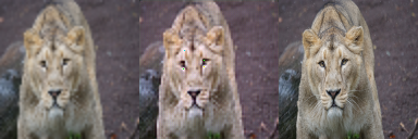
Visualize the dataset
Let’s visualize the dataset downloaded and scaled:
img_lr, img_hr = next(iter(train_ds))

lr = Image.fromarray(np.array(img_lr)[0].astype(np.uint8))
lr = lr.resize([256, 256])
display(lr)

hr = Image.fromarray(np.array(img_hr)[0].astype(np.uint8))
hr = hr.resize([256, 256])
display(hr)
 |
 |
We will first define the generator architecture, the discriminator architecture and the loss functions; and then put everything together to form the ESRGAN model.
Generator - as with most GAN generators, the ESRGAN generator upsamples the input a few times. What makes it different is the Residual-in-Residual Block (RRDB) without batch normalization.
In the generator we define the function for creating the Conv block, Dense block, RRDB block for upsampling. Then we define a function to create the generator network as follows with Keras Functional API:
def generator_network(filter=32,
                     trunk_size=Params['trunk_size'],
                     out_channels=3):
 lr_input = layers.Input(shape=(None, None, 3))

 x = layers.Conv2D(filter, kernel_size=[3,3], strides=[1,1],
                   padding='same', use_bias=True)(lr_input)
 x = layers.LeakyReLU(0.2)(x)
  ref = x
 for i in range(trunk_size):
     x = rrdb(x)

 x = layers.Conv2D(filter, kernel_size=[3,3], strides=[1,1],
                   padding='same', use_bias = True)(x)
 x = layers.Add()([x, ref])

 x = upsample(x, filter)
 x = upsample(x, filter)
  x = layers.Conv2D(filter, kernel_size=3, strides=1,
                   padding='same', use_bias=True)(x)
 x = layers.LeakyReLU(0.2)(x)
 hr_output = layers.Conv2D(out_channels, kernel_size=3, strides=1,
                           padding='same', use_bias=True)(x)

 model = tf.keras.models.Model(inputs=lr_input, outputs=hr_output)
 return model
Discriminator
The discriminator is a fairly straightforward CNN with Conv2D, BatchNormalization, LeakyReLU and Dense layers. Again, with the Keras Functional API.
def discriminator_network(filters = 64, training=True):
 img = layers.Input(shape = (Params['hr_dimension'], Params['hr_dimension'], 3))

 x = layers.Conv2D(filters, [3,3], 1, padding='same', use_bias=False)(img)
 x = layers.BatchNormalization()(x)
 x = layers.LeakyReLU(alpha=0.2)(x)

 x = layers.Conv2D(filters, [3,3], 2, padding='same', use_bias=False)(x)
 x = layers.BatchNormalization()(x)
 x = layers.LeakyReLU(alpha=0.2)(x)

 x = _conv_block_d(x, filters *2)
 x = _conv_block_d(x, filters *4)
 x = _conv_block_d(x, filters *8)
  x = layers.Flatten()(x)
 x = layers.Dense(100)(x)
 x = layers.LeakyReLU(alpha=0.2)(x)
 x = layers.Dense(1)(x)

 model = tf.keras.models.Model(inputs = img, outputs = x)
 return model
Loss Functions
The ESRGAN model makes use of three loss functions to ensure the balance between visual quality and metrics such as Peak Signal-to- Noise Ratio (PSNR) and encourages the generator to produce more realistic images with natural textures:
Let’s dive deeper into the adversarial loss here since this is the most complex one and it’s a function added to the TF-GAN library as part of the project.
In GANs the discriminator network classifies the input data as real or fake. The generator is trained to generate fake data and fool the discriminator into mistakenly classifying it as real. As the generator increases the probability of fake data being real, the probability of real data being real should also decrease. This was a missing property of standard GANs as pointed out in this paper, and the relativistic discriminator was introduced to overcome this issue. The relativistic average discriminator estimates the probability that the given real data is more realistic than fake data, on average. This improves the quality of generated data and the stability of the model while training. In the TF-GAN library, see relativistic_generator_loss and relativistic_discriminator_loss for the implementation of this loss function.
def ragan_generator_loss(d_real, d_fake):
 real_logits = d_real - tf.reduce_mean(d_fake)
 fake_logits = d_fake - tf.reduce_mean(d_real)
  real_loss = tf.reduce_mean(tf.nn.sigmoid_cross_entropy_with_logits(
     labels=tf.zeros_like(real_logits), logits=real_logits))
 fake_loss = tf.reduce_mean(tf.nn.sigmoid_cross_entropy_with_logits(
     labels=tf.ones_like(fake_logits), logits=fake_logits))

 return real_loss + fake_loss

def ragan_discriminator_loss(d_real, d_fake):
 def get_logits(x, y):
   return x - tf.reduce_mean(y)
  real_logits = get_logits(d_real, d_fake)
 fake_logits = get_logits(d_fake, d_real)

 real_loss = tf.reduce_mean(tf.nn.sigmoid_cross_entropy_with_logits(
         labels=tf.ones_like(real_logits), logits=real_logits))
 fake_loss = tf.reduce_mean(tf.nn.sigmoid_cross_entropy_with_logits(
     labels=tf.zeros_like(fake_logits), logits=fake_logits))

 return real_loss + fake_loss
The ESRGAN model is trained in two phases:
If starting from scratch, phase-1 training can be completed within an hour on a free colab TPU, whereas phase-2 can take around 2-3 hours to get good results. As a result saving the weights/checkpoints are important steps during training.
Here are the steps of phase 1 training:
In this phase of training:
Then we define the training step as follows:
Please refer to the Colab notebook for the complete code implementation.
During training we visualize the 3 images: LR image, HR image (generated), HR image (training data), and these metrics: generator loss, discriminator loss and PSNR.
step 0
Generator Loss = 0.636057436466217
Disc Loss = 0.0191921629011631
PSNR : 20.95576286315918
Here are some more results at the end of the training which look pretty good.


Now that training has completed, we will evaluate the ESRGAN model with 3 metrics: Fréchet Inception Distance (FID), Inception Scores and Peak signal-to-noise ratio (PSNR).
FID and Inception Scores are two common metrics used to evaluate the performance of a GAN model. Peak Signal-to- Noise Ratio (PSNR) is used to quantify the similarity between two images and is used for benchmarking super resolution models.
Instead of writing the code from scratch to calculate each of the metrics, we are using the TF-GAN library to evaluate our GAN implementation with ease for FID and Inception Scores. Then we make use of the `tf.image` module to calculate PSNR values for evaluating the super resolution algorithm.
Why do we need the TF-GAN library for evaluation?
Standard evaluation metrics for GANs such as Inception Scores, Frechet Distance or Kernel Distance are available inside TF-GAN Evaluation. Various implementations of such metrics can be prone to errors and this can result in unreliable evaluation scores. By using TF-GAN, such errors can be avoided and GAN evaluations can be made easy. For evaluating the ESRGAN model we have made use of the Inception Score (tfgan.eval.inception_score) and Frechet Distance Score (tfgan.eval.frechet_inception_distance) from the TF-GAN library.
Here is how we use tf-gan for evaluation in code.
First we need to install the tf-gan library which should have been part of the imports at the beginning of the notebook. Then we import the library.
!pip install tensorflow-gan
import tensorflow_gan as tfgan
Now we are ready to use the library for the ESRGAN evaluation!
Fréchet inception distance (FID)
@tf.function
def get_fid_score(real_image, gen_image):
 size = tfgan.eval.INCEPTION_DEFAULT_IMAGE_SIZE

 resized_real_images = tf.image.resize(real_image, [size, size], method=tf.image.ResizeMethod.BILINEAR)
 resized_generated_images = tf.image.resize(gen_image, [size, size], method=tf.image.ResizeMethod.BILINEAR)
  num_inception_images = 1
 num_batches = Params['batch_size'] // num_inception_images
  fid = tfgan.eval.frechet_inception_distance(resized_real_images, resized_generated_images, num_batches=num_batches)
 return fid
@tf.function
def get_inception_score(images, gen, num_inception_images = 8):
 size = tfgan.eval.INCEPTION_DEFAULT_IMAGE_SIZE
 resized_images = tf.image.resize(images, [size, size], method=tf.image.ResizeMethod.BILINEAR)

 num_batches = Params['batch_size'] // num_inception_images
 inc_score = tfgan.eval.inception_score(resized_images, num_batches=num_batches)

return inc_scoredef get_psnr(real, generated):
psnr_value = tf.reduce_mean(tf.image.psnr(generated, real, max_val=256.0))
return psnr_value
Here is the Google Summer of Code 2021 experience in our own words:
Nived
As a student, Google Summer of Code gave me an opportunity to participate in exciting open source projects for TensorFlow and the mentorship that I got during this period was invaluable. I got to learn a lot about implementing various GAN models, writing tutorial notebooks, using Cloud TPUs for training models and using tools such as Google Cloud Platform. I received a lot of support from Margaret and Joel throughout the program which kept the project on track. From the beginning their suggestions helped define the project scope and during the coding period, Margaret and I met on a weekly basis to clear all my doubts and solve various issues that I was facing. Joel also helped in reviewing all the PRs made to the TF-GAN library. GSoC is indeed a great way of getting involved with various interesting TensorFlow libraries and I look forward to continuing making valuable contributions to the community.
Margaret
As the project mentor, I have been involved since the project selection phase. Mentoring Nived and collaborating with Joel on TF-GAN has been a fulfilling experience. Nived has done an excellent job implementing the ESRGAN paper with TensorFlow 2 and TF-GAN. Nived and I spent a lot of time looking at the various text-to-image GANs to choose one that can potentially be implemented during the GSoC timeframe. Aside from writing the ESRGAN tutorial, he made great progress on ControlGAN for text-to-image generation. I hope this project helps others to learn how to use the TF-GAN library and contribute to TF-GAN and other open source TensorFlow projects.
Joel
As an unofficial technical mentor, I was impressed how independently and effectivly Nived worked. I felt more like I was working with a junior colleague than an intern, in that I helped give technical and project pointers, but ultimately Nived made the decisions. I think the impressive results reflect this: Nived owned the project, and I think as a result the example and Colab are more well-written and cohesive than they otherwise might have been. Furthermore, Nived successfully navigated the multi-timezone reality that is working-from-home!
During the GSoC coding period the implementation of the ESRGAN model was completed and the Python code and Colab notebooks were merged to the TF-GAN repo. The implementation of the ControlGAN model for text-to-image generation is still in progress. Once the implementation of ControlGAN is completed, we plan to extend it to serve some real-world applications in areas such as art generation or image editing. We are also planning to write tutorials to explore different models that solve the task of text-to-image translation.
If you want to contribute to TF-GAN, you can reach out to `tfgan-users@google.com` to propose a project or addition. Unless you've contributed to OSS Google projects before, it's usually a good idea to check with someone before submitting a large pull request. We look forward to seeing your contributions and working with you!
We would like to thank the GSoC program committee and their support, in particular Josh Gordon from the TensorFlow team.
Many thanks to the support of the Machine Learning (ML) Google Developer Expert (GDE) program, Google Cloud Platform and TensorFlow Research Cloud.

січня 10, 2022 — Posted by Nived P A, Margaret Maynard-Reid, Joel ShorGoogle Summer of Code is a program that brings student developers into open-source projects each summer. This article describes enhancements made to the TensorFlow GAN library (TF-GAN) last summer that were proposed by Nived PA, an undergraduate student of Amrita School of Engineering. The goal of Nived’s project was to improve the TF-GAN libra…


