Posted by Hugo Zanini, Data Product Manager
Last year, I published an article on how to train custom object detection in the browser using TensorFlow.js. This received lots of interest from developers from all over the world who tried to apply the solution to their personal or business projects.While answering reader’s questions on my first article, I noticed a few difficulties in adapting our solution to large datasets, and deploying the resulting model in production using the new version of TensorFlow.js.
Therefore, the goal of this article is to share a solution for a well-known problem in the consumer packaged goods (CPG) industry: real-time and offline SKU detection using TensorFlow.js.

| Offline SKU detection running in real time on a smartphone using TensorFlow.js |
The problem
Items consumed frequently by consumers (foods, beverages, household products, etc) require an extensive routine of replenishment and placement of those products at their point of sale (supermarkets, convenience stores, etc).
Over the past few years, researchers have shown repeatedly that about two-thirds of purchase decisions are made after customers enter the store. One of the biggest challenges for consumer goods companies is to guarantee the availability and correct placement of their product in-stores.
At stores, teams organize the shelves based on marketing strategies, and manage the level of products in the stores. The people working on these activities may count the number of SKUs of each brand in a store to estimate product stocks and market share, and help to shape marketing strategies.
These estimations though are very time-consuming. Taking a photo and using an algorithm to count the SKUs on the shelves to calculate a brand’s market share could be a good solution.
To use an approach like that, the detection should run in real-time such that as soon as you point a phone camera to the shelf, the algorithm recognizes the brands and calculates the market shares. And, as the internet inside the stores is generally limited, the detection should work offline.

| Example workflow |
This post is going to show how to implement the real-time and offline image recognition solution to identify generic SKUs using the SKU110K dataset and the MobileNetV2 network.
Due to the lack of a public dataset with labeled SKUs of different brands, we’re going to create a generic algorithm, but all the instructions can be applied in a multiclass problem.
As with every machine learning flow, the project will be divided into four steps, as follows:

| Object Detection Model Production Pipeline |
Preparing the data
The first step to training a good model is to gather good data. As mentioned before, this solution is going to use a dataset of SKUs in different scenarios. The purpose of SKU110K was to create a benchmark for models capable of recognizing objects in densely packed scenes.
The dataset is provided in the Pascal VOC format and has to be converted to tf.record. The script to do the conversion is available here and the tf.record version of the dataset is also available in my project repository. As mentioned before, SKU110K is a large and very challenging dataset to work with. It contains many objects, often looking similar or even identical, positioned in close proximity.
To work with this dataset, the neural network chosen has to be very effective in recognizing patterns and be small enough to run in real-time in TensorFlow.js.
Choosing the model
There are a variety of neural networks capable of solving the SKU detection problem. But, the architectures that easily achieve a high level of precision are very dense and don't have reasonable inference times when converted to TensorFlow.js to run in real-time.
Because of that, the approach here is going to be to focus on optimizing a mid-level neural network to achieve reasonable precision working on densely packed scenes and run the inferences in real-time. Analyzing the TensorFlow 2.0 Detection Model Zoo, the challenge will be to try to solve the problem using the lighter single-shot model available: SSD MobileNet v2 320x320 which seems to fit the criteria required. The architecture is proven to be able to recognize up to 90 classes and can be trained to identify different SKUs.
Training the model
With a good dataset and the model selected, it’s time to think about the training process. TensorFlow 2.0 provides an Object Detection API that makes it easy to construct, train, and deploy object detection models. In this project, we’re going to use this API and train the model using a Google Colaboratory Notebook. The remainder of this section explains how to set up the environment, the model selection, and training. If you want to jump straight to the Colab Notebook, click here.
Setting up the environment
Create a new Google Colab notebook and select a GPU as the hardware accelerator:
Runtime > Change runtime type > Hardware accelerator: GPU
Clone, install, and test the TensorFlow Object Detection API:
Next, download and extract the dataset using the following commands:
Setting up the training pipeline
We’re ready to configure the training pipeline. TensorFlow 2.0 provides pre-trained weights for the SSD Mobilenet v2 320x320 on the COCO 2017 Dataset, and they are going to be downloaded using the following commands:
The downloaded weights were pre-trained on the COCO 2017 Dataset, but the focus here is to train the model to recognize one class so these weights are going to be used only to initialize the network — this technique is known as transfer learning, and it’s commonly used to speed up the learning process.
The last step is to set up the hyperparameters on the configuration file that is going to be used during the training. Choosing the best hyperparameters is a task that requires some experimentation and, consequently, computational resources.
I took a standard configuration of MobileNetV2 parameters from the TensorFlow Models Config Repository and performed a sequence of experiments (thanks Google Developers for the free resources) to optimize the model to work with densely packed scenes on the SKU110K dataset. Download the configuration and check the parameters using the code below.
With the parameters set, start the training by executing the following command:
To identify how well the training is going, we use the loss value. Loss is a number indicating how bad the model’s prediction was on the training samples. If the model’s prediction is perfect, the loss is zero; otherwise, the loss is greater. The goal of training a model is to find a set of weights and biases that have low loss, on average, across all examples (Descending into ML: Training and Loss | Machine Learning Crash Course).
The training process was monitored through Tensorboard and took around 22h to finish on a 60GB machine using an NVIDIA Tesla P4. The final losses can be checked below

| Total training loss |
Validate the model
Now let’s evaluate the trained model using the test data:
The evaluation was done across 2740 images and provides three metrics based on the COCO detection evaluation metrics: precision, recall, and loss (Classification: Precision and Recall | Machine Learning Crash Course). The same metrics are available via Tensorboard and can be analyzed in an easier way
%load_ext tensorboard
%tensorboard --logdir '/content/training/'
You can then explore all training and evaluation metrics.

| Main evaluation metrics |
Exporting the model
Now that the training is validated, it’s time to export the model. We’re going to convert the training checkpoints to a protobuf (pb) file. This file is going to have the graph definition and the weights of the model.
As we’re going to deploy the model using TensorFlow.js and Google Colab has a maximum lifetime limit of 12 hours, let’s download the trained weights and save them locally. When running the command files.download("/content/saved_model.zip"), the Colab will prompt the file download automatically.
Deploying the model
The model is going to be deployed in a way that anyone can open a PC or mobile camera and perform inference in real-time through a web browser. To do that, we’re going to convert the saved model to the TensorFlow.js layers format, load the model in a JavaScript application and make everything available on CodeSandbox.
Converting the model
At this point, you should have something similar to this structure saved locally:
%MD
├── inference-graph
│ ├── saved_model
│ │ ├── assets
│ │ ├── saved_model.pb
│ │ ├── variables
│ │ ├── variables.data-00000-of-00001
│ │ └── variables.index
Before we start, let’s create an isolated Python environment to work in an empty workspace and avoid any library conflict. Install virtualenv and then open a terminal in the inference-graph folder and create and activate a new virtual environment:
virtualenv -p python3 venv
source venv/bin/activate
Install the TensorFlow.js converter:
pip install tensorflowjs[wizard]
Start the conversion wizard:
tensorflowjs_wizard
Now, the tool will guide you through the conversion, providing explanations for each choice you need to make. The image below shows all the choices that were made to convert the model. Most of them are the standard ones, but options like the shard sizes and compression can be changed according to your needs.
To enable the browser to cache the weights automatically, it’s recommended to split them into shard files of around 4MB. To guarantee that the conversion is going to work, don’t skip the op validation as well, not all TensorFlow operations are supported so some models can be incompatible with TensorFlow.js — See this list for which ops are currently supported on the various backends that TensorFlow.js executes on such as WebGL, WebAssembly, or plain JavaScript.
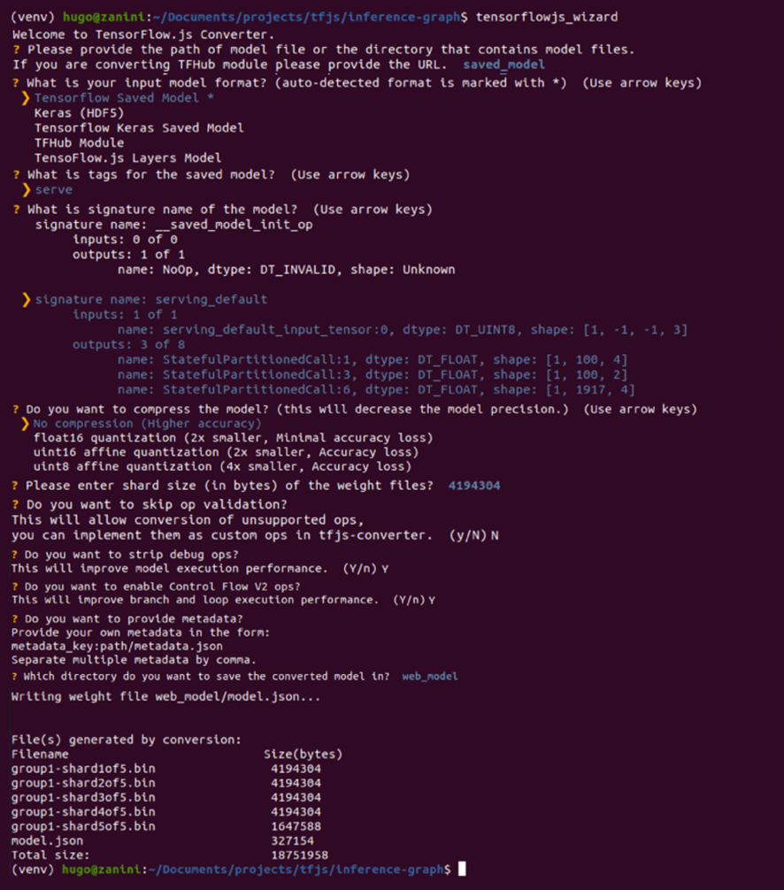
Model conversion using TensorFlow.js Converter (Full resolution image here) |
If everything works well, you’re going to have the model converted to the TensorFlow.js layers format in the web_model directory. The folder contains a model.json file and a set of sharded weights files in a binary format. The model.json has both the model topology (aka “architecture” or “graph”: a description of the layers and how they are connected) and a manifest of the weight files (Lin, Tsung-Yi, et al). The contents of the web_model folder currently contains the files shown below:
└ web_model
  ├── group1-shard1of5.bin
  ├── group1-shard2of5.bin
  ├── group1-shard3of5.bin
  ├── group1-shard4of5.bin
  ├── group1-shard5of5.bin
  └── model.json
Configuring the application
The model is ready to be loaded in JavaScript. I’ve created an application to perform inference directly from the browser. Let’s clone the repository to figure out how to use the converted model in real-time. This is the project structure:
├── models
│	├── group1-shard1of5.bin
│	├── group1-shard2of5.bin
│	├── group1-shard3of5.bin
│	├── group1-shard4of5.bin
│	├── group1-shard5of5.bin
│	└── model.json
├── package.json
├── package-lock.json
├── public
│   └── index.html
├── README.MD
└── src
	├── index.js
	└── styles.css
For the sake of simplicity, I have already provided a converted SKU-detector model in the model's folder. However, let’s put the web_model generated in the previous section in the models folder and test it.
Next, install the http-server:
npm install http-server -g
Go to the models folder and run the command below to make the model available at http://127.0.0.1:8080 . This is a good choice when you want to keep the model weights in a safe place and control who can request inferences to it. The -c1 parameter is added to disable caching, and the --cors flag enables cross-origin resource sharing allowing the hosted files to be used by the client-side JavaScript for a given domain.
http-server -c1 --cors .
Alternatively, you can upload the model files somewhere else - even on a different domain if needed. In my case, I chose my own Github repo and referenced the model.json folder URL in the load_model function as shown below:
async function load_model() {
	// It's possible to load the model locally or from a repo.
	// Load from localhost locally:
      const model = await loadGraphModel("http://127.0.0.1:8080/model.json");
	// Or Load from another domain using a folder that contains model.json.
      // const model = await loadGraphModel("https://github.com/hugozanini/realtime-sku-detection/tree/web");
	return model;
}
This is a good option because it gives more flexibility to the application and makes it easier to run on public web servers.
Pick one of the methods to load the model files in the function load_model (lines 10–15 in the file src>index.js).
When loading the model, TensorFlow.js will perform the following requests:
GET /model.json
GET /group1-shard1of5.bin
GET /group1-shard2of5.bin
GET /group1-shard3of5.bin
GET /group1-shardo4f5.bin
GET /group1-shardo5f5.bin
Publishing in CodeSandbox
CodeSandbox is a simple tool for creating web apps where we can upload the code and make the application available for everyone on the web. By uploading the model files in a GitHub repo and referencing them in the load_model function, we can simply log into CodeSandbox, click on New project > Import from Github, and select the app repository.
Wait some minutes to install the packages and your app will be available at a public URL that you can share with others. Click on Show > In a new window and a tab will open with a live preview. Copy this URL and paste it in any web browser (PC or Mobile) and your object detection will be ready to run. A ready to use project can be found here as well if you prefer.
ConclusionBesides the precision, an interesting part of these experiments is the inference time — everything runs in real-time in the browser via JavaScript. SKU detection models running in the browser, even offline, and using few computational resources is a must in many consumer packaged goods company applications, along with other industries too.
Enabling a Machine Learning solution to run on the client-side is a key step to guarantee that the models are being used effectively at the point of interaction with minimal latency and solve the problems when they happen: right in the user's hand.
Deep learning should not be costly and should be used beyond just research, for real world use cases, which JavaScript is great for production deployments. I hope this article will serve as a basis for new projects involving Computer Vision, TensorFlow, and create an easier flow between Python and Javascript.
If you have any questions or suggestions you can reach me on Twitter.
Thanks for reading!
Acknowledgments
I’d like to thank the Google Developers Group, for providing all the computational resources for training the models, and the authors of the SKU 110K Dataset, for creating and open-sourcing the dataset used in this project.

mayo 23, 2022 — Posted by Hugo Zanini, Data Product Manager Last year, I published an article on how to train custom object detection in the browser using TensorFlow.js. This received lots of interest from developers from all over the world who tried to apply the solution to their personal or business projects.While answering reader’s questions on my first article, I noticed a few difficulties in adapting our s…


