Posted by Chansung Park and Sayak Paul (ML and Cloud GDEs)
Generative AI models like Stable Diffusion1 that lets anyone generate high-quality images from natural language text prompts enable different use cases across different industries. These types of models allow people to generate these images not only from images but also condition them with other inputs such as segmentation maps, other images, depth maps, etc. In many ways, an end Stable Diffusion system (such as this) is often very complete. One gives a free-form text prompt to start the generation process, and in the end, an image (or any data in the continuous modality) gets generated.
In this post, we discuss how TensorFlow Serving (TF Serving) and Google Kubernetes Engine (GKE) can serve such a system with online deployment. Stable Diffusion is just one example of many such systems that TF and GKE can serve with online deployment. We start by breaking down Stable Diffusion into main components and how they influence the subsequent consideration for deployment. Then we dive deep into the deployment-specific bits such as TF Serving deployment and k8s cluster configuration. Our code is open-sourced in this repository.
Let’s dive in.
Stable Diffusion, is comprised of three sub-models:
- CLIP’s text tower as the Text Encoder,
- Diffusion Model (UNet), and
- Decoder of a Variational Autoencoder
When generating images from an input text prompt, the prompt is first embedded into a latent space with the text encoder. Then an initial noise is sampled, which is fed to the Diffusion model along with the text embeddings. This noise is then denoised using the Diffusion model in a continuous manner – the so-called “diffusion” process. The output of this step is a denoise latent, and it is fed to the Decoder for final image generation. Figure 1 provides an overview.
(For a more complete overview of Stable Diffusion, refer to this post.)
 |
| Figure 1. Stable Diffusion Architecture |
As mentioned above, three sub-models of Stable Diffusion work in a sequential manner. It’s common to run all three models on a single server (which constructs the end Stable Diffusion system) and serve the system as a whole.
However, because each component is a standalone deep learning model, each one could be served independently. This is particularly useful because each component has different hardware requirements. This can also have potentially improved resource utilization. The text encoder can still be run on moderate CPUs, whereas the other two should be run on GPUs, especially the UNet should be served with larger size GPUs (~3.4 GBs in size).
 |
| Figure 2. Decomposing Stable Diffusion in three parts |
Figure 2 shows the Stable Diffusion serving architecture that packages each component into a separate container with TensorFlow Serving, which runs on the GKE cluster. This separation brings more control when we think about local compute power and the nature of fine-tuning of Stable Diffusion as shown in Figure 3.
NOTE: TensorFlow Serving is a flexible, high-performance serving system for machine learning models, designed for production environments, which is widely adopted in industry. The benefits of using it include GPU serving support, dynamic batching, model versioning, RESTful and gRPC APIs, to name but a few.
In modern personal devices such as desktops and mobile phones, it is common that they are equipped with moderate CPUs and sometimes GPU/NPUs. In this case, we could selectively run the UNet and/or Decoder in the cloud using high capacity GPUs while running the text encoder locally on the user’s device. In general, this approach allows us to flexibly architect the Stable Diffusion system in a way to maximize the resource utilization.
 |
| Figure 3. Flexible serving structure of Stable Diffusion |
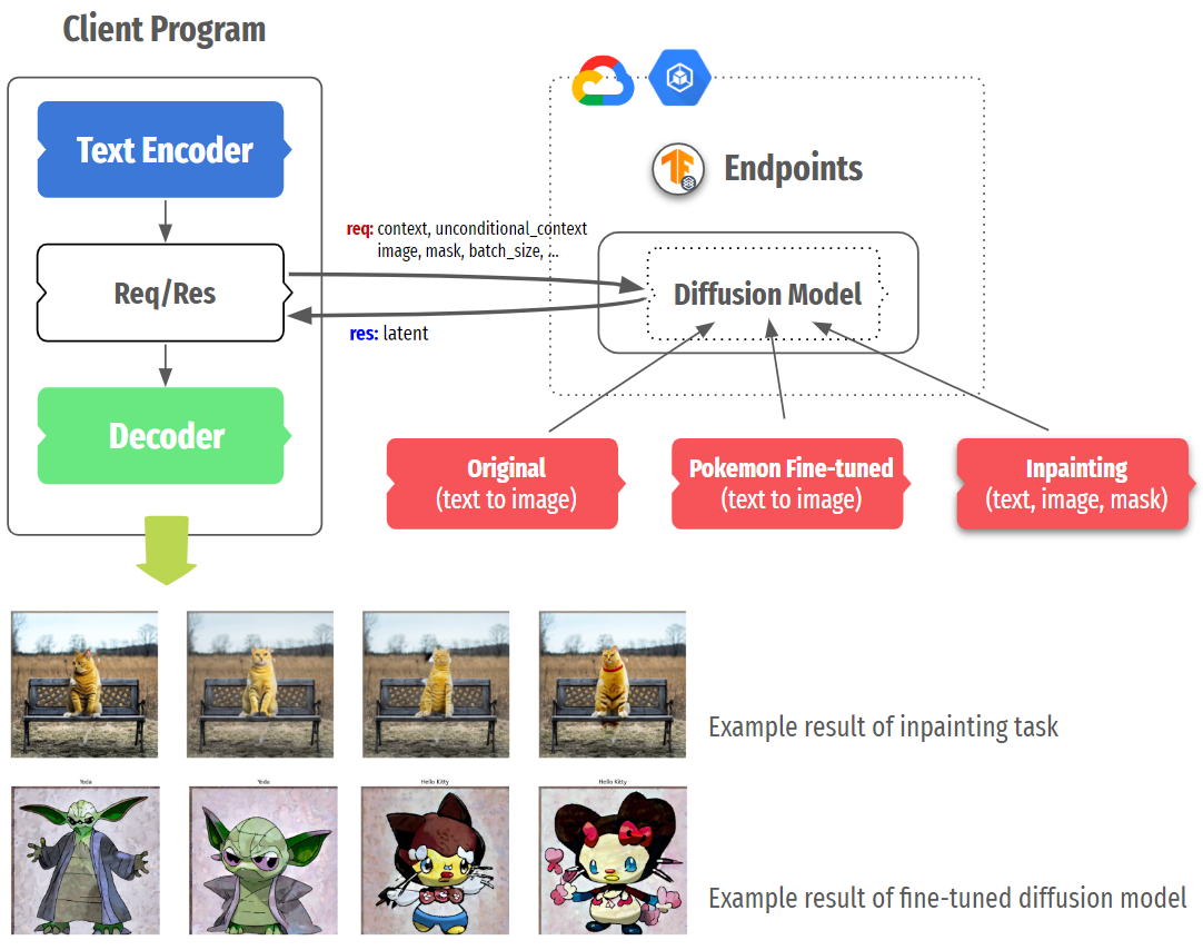
One more scenario to consider is fine-tuned Stable Diffusion. Many variations such as DreamBooth, Textual Inversion, or style transfer have shown that modifying only one or two components (usually Text Encoder and UNet) can generate images with new concepts or different styles. In this case, we could selectively deploy more of certain fine-tuned models on separate instances or replace existing models without touching other parts.
In order to serve a TensorFlow/Keras model with TF Serving, it should be saved in the SavedModel format. After that, the model can be served by TF Serving, a high-performance serving system for machine learning models, specially designed for production environments. The potentially non-trivial parts of making a SavedModel could be divided into three parts:
- defining an appropriate input signature specification of the underlying model,
- performing computations with the underlying model so that everything can be compiled in native TensorFlow, and
- including most of the pre and post-processing operations within the
SavedModelgraph itself to reduce training/serving skew (this is optional, but highly recommended).
To make the Stable Diffusion class shipped in KerasCV compatible with TF Serving, we need to first isolate the sub-networks (as mentioned above) of the class. Recall that we have got three sub-networks here: text encoder, diffusion model, and a decoder. We then have to serialize these networks as SavedModels.
A diffusion system also involves iterative sampling where a noise vector is gradually turned into an image. KerasCV’s Stable Diffusion class implements the sampling process with non-TensorFlow operations. So, we need to eliminate those operations and ensure that it’s implemented in pure TensorFlow so that there is end-to-end compatibility. This was the single most challenging aspect for us in the whole project.
Since the serialization of the text encoder and the decoder is straightforward, we’ll skip that in this post and instead, focus on the serialization of the diffusion model, including the sampling process. You can find an end-to-end notebook here.
We start by defining an input signature dictionary for the SavedModel to be serialized. In this case, the inputs consist:
context, that denotes embeddings of the input text prompt extracted with the text encoderunconditional_context, that denotes the embeddings of a so-called “null prompt” (see classifier-free guidance)num_steps, that denotes the number of sampling steps for the reverse diffusion processbatch_size, that denotes the number of images to be returned
from keras_cv.models.stable_diffusion.constants import ALPHAS_CUMPROD_TF
import tensorflow as tf

IMG_HEIGHT = 512
IMG_WIDTH = 512
MAX_PROMPT_LENGTH = 77
ALPHAS_CUMPROD_TF = tf.constant(ALPHAS_CUMPROD_TF)
UNCONDITIONAL_GUIDANCE_SCALE = 7.5
HIDDEN_DIM = 768
SEED = None


signature_dict = {
    "context": tf.TensorSpec(shape=[None, MAX_PROMPT_LENGTH, HIDDEN_DIM], dtype=tf.float32, name="context"),
    "unconditional_context": tf.TensorSpec(
        shape=[None, MAX_PROMPT_LENGTH, HIDDEN_DIM], dtype=tf.float32, name="unconditional_context"
    ),
    "num_steps": tf.TensorSpec(shape=[], dtype=tf.int32, name="num_steps"),
    "batch_size": tf.TensorSpec(shape=[], dtype=tf.int32, name="batch_size"),
} |
Next up, we implement the iterative reverse diffusion process that involves the pre-trained diffusion model. diffusion_model_exporter() takes this model as an argument. serving_fn() is the function we use for exporting the final SavedModel. Most of this code is taken from the original KerasCV implementation here, except it has got all the operations implemented in native TensorFlow.
def diffusion_model_exporter(model: tf.keras.Model):
    @tf.function
    def get_timestep_embedding(timestep, batch_size, dim=320, max_period=10000):
        ...
    @tf.function(input_signature=[signature_dict])
    def serving_fn(inputs):
        img_height = tf.cast(tf.math.round(IMG_HEIGHT / 128) * 128, tf.int32)
        img_width = tf.cast(tf.math.round(IMG_WIDTH / 128) * 128, tf.int32)

        batch_size = inputs["batch_size"]
        num_steps = inputs["num_steps"]

        context = inputs["context"]
        unconditional_context = inputs["unconditional_context"]

        latent = tf.random.normal((batch_size, img_height // 8, img_width // 8, 4))

        timesteps = tf.range(1, 1000, 1000 // num_steps)
        alphas = tf.map_fn(lambda t: ALPHAS_CUMPROD_TF[t], timesteps, dtype=tf.float32)
        alphas_prev = tf.concat([[1.0], alphas[:-1]], 0)

        index = num_steps - 1
        latent_prev = None
        for timestep in timesteps[::-1]:
            latent_prev = latent
            t_emb = get_timestep_embedding(timestep, batch_size)
            unconditional_latent = model(
                [latent, t_emb, unconditional_context], training=False
            )
            latent = model([latent, t_emb, context], training=False)
            latent = unconditional_latent + UNCONDITIONAL_GUIDANCE_SCALE * (
                latent - unconditional_latent
            )
            a_t, a_prev = alphas[index], alphas_prev[index]
            pred_x0 = (latent_prev - tf.math.sqrt(1 - a_t) * latent) / tf.math.sqrt(a_t)
            latent = (
                latent * tf.math.sqrt(1.0 - a_prev) + tf.math.sqrt(a_prev) * pred_x0
            )
            index = index - 1

        return {"latent": latent}

return serving_fn |
Then, we can serialize the diffusion model as a SavedModel like so:
tf.saved_model.save(
    diffusion_model,
    path_to_serialize_the_model,
    signatures={"serving_default": diffusion_model_exporter(diffusion_model)},
) |
Here, diffusion_model is the pre-trained diffusion model initialized like so:
from keras_cv.models.stable_diffusion.diffusion_model import DiffusionModel
diffusion_model = DiffusionModel(IMG_HEIGHT, IMG_WIDTH, MAX_PROMPT_LENGTH) |
Once you have successfully created TensorFlow SavedModels, it is quite straightforward to deploy them with TensorFlow Serving to a GKE cluster in the following steps.
- Write Dockerfiles which are based on the TensorFlow Serving base image
- Create a GKE cluster with accelerators attached
- Apply NVIDIA GPU driver installation daemon to install the driver on each node
- Write deployment manifests with GPU allocation
- Write service manifests to expose the deployments
- Apply all the manifests
The easiest way to wrap a SavedModel in TensorFlow Serving is to leverage the pre-built TensorFlow Serving Docker images. Depending on the configuration of the machine that you’re deploying to, you should choose either tensorflow/serving:latest or tensorflow/serving:latest-gpu. Because all the steps besides GPU-specific configuration are the same, we will explain this section with an example of the Diffusion Model part only.
By default, TensorFlow Serving recognizes embedded models under /models, so the entire SavedModel folder tree should be placed inside /models/{model_name}/{version_num}. A single TensorFlow Serving instance can serve multiple versions of multiple models, so that is why we need such a {model_name}/{version_num} folder structure. A SavedModel can be exposed as an API by setting a special environment variable MODEL_NAME, which is used for TensorFlow Serving to look for which model to serve.
FROM tensorflow/serving:latest-gpu
...
RUN mkdir -p /models/text-encoder/1
RUN cp -r tfs-diffusion-model/* /models/diffusion-model/1/
ENV MODEL_NAME=diffusion-model
... |
Next step is to create a GKE cluster. You can do this by using either Google Cloud Console or gcloud container CLI as below. If you want accelerators available on each node, you can specify how many of which GPUs to be attached with --accelerator=type={ACCEL_TYPE}, count={ACCEL_NUM} option.
$ gcloud container clusters create {CLUSTER_NAME} \
  --machine-type={MACHINE_TYPE} \                     # n1-standard-4
  --accelerator=type={GPU_TYPE},count={GPU_NUM} \     # nvidia-tesla-v100, 1
... |
Once the cluster is successfully created, and if the nodes in the cluster have accelerators attached, an appropriate driver for them should be installed correctly. This is done by running a special DaemonSet, which tries to install the driver on each node. If the driver has not been successfully installed, and if you try to apply Deployment manifests requiring accelerators, the status of the pod remains as Pending.
DRIVER_URL = https://raw.githubusercontent.com/GoogleCloudPlatform/container-engine-accelerators/master/nvidia-driver-installer/cos/daemonset-preloaded.yaml
kubectl apply -f $DRIVER_URL |
Make sure all the pods are up and running with kubectl get pods -A command. Then, we are ready to apply prepared Deployment manifests. Below is an example of the Deployment manifest for the Diffusion Model. The only consideration you need to take is to specify which resource the pods of the Deployment should consume. Because the Diffusion Model needs to be run on accelerators, resources:limits:nvidia.com/gpu: {ACCEL_NUM} should be set.
Furthermore, if you want to expose gRPC and RestAPI at the same time, you need to set containerPort for both. TensorFlow Serving exposes the two endpoints via 8500 and 8501, respectively, by default, so both ports should be specified.
apiVersion: apps/v1
kind: Deployment
...
    spec:
      containers:
      - image: {IMAGE_URI}
...
        args: ["--rest_api_timeout_in_ms=1200000"]
        ports:
        - containerPort: 8500
          name: grpc
        - containerPort: 8501
          name: restapi
        resources:
          limits:
nvidia.com/gpu: 1 |
One more thing to note is that --rest_api_timeout_in_ms flag is set in args with a huge number. It takes a long time for heavy models to run inference. Since the flag is set to 5,000ms by default which is 5 seconds, sometimes timeout occurs before the inference is done. You can experimentally find out the right number, but we simply set this with a high enough number to demonstrate this project smoothly.
The final step is to apply prepared manifest files to the provisioned GKE cluster. This could be easily done with the kubectl apply -f command. Also, you could apply Service and Ingress depending on your needs. Because we simply used vanilla LoadBalancer type of Service for demonstration purposes, it is not listed in this blog. You can find all the Dockerfiles, and the Deployment and Service manifests in the accompanying GitHub repository.
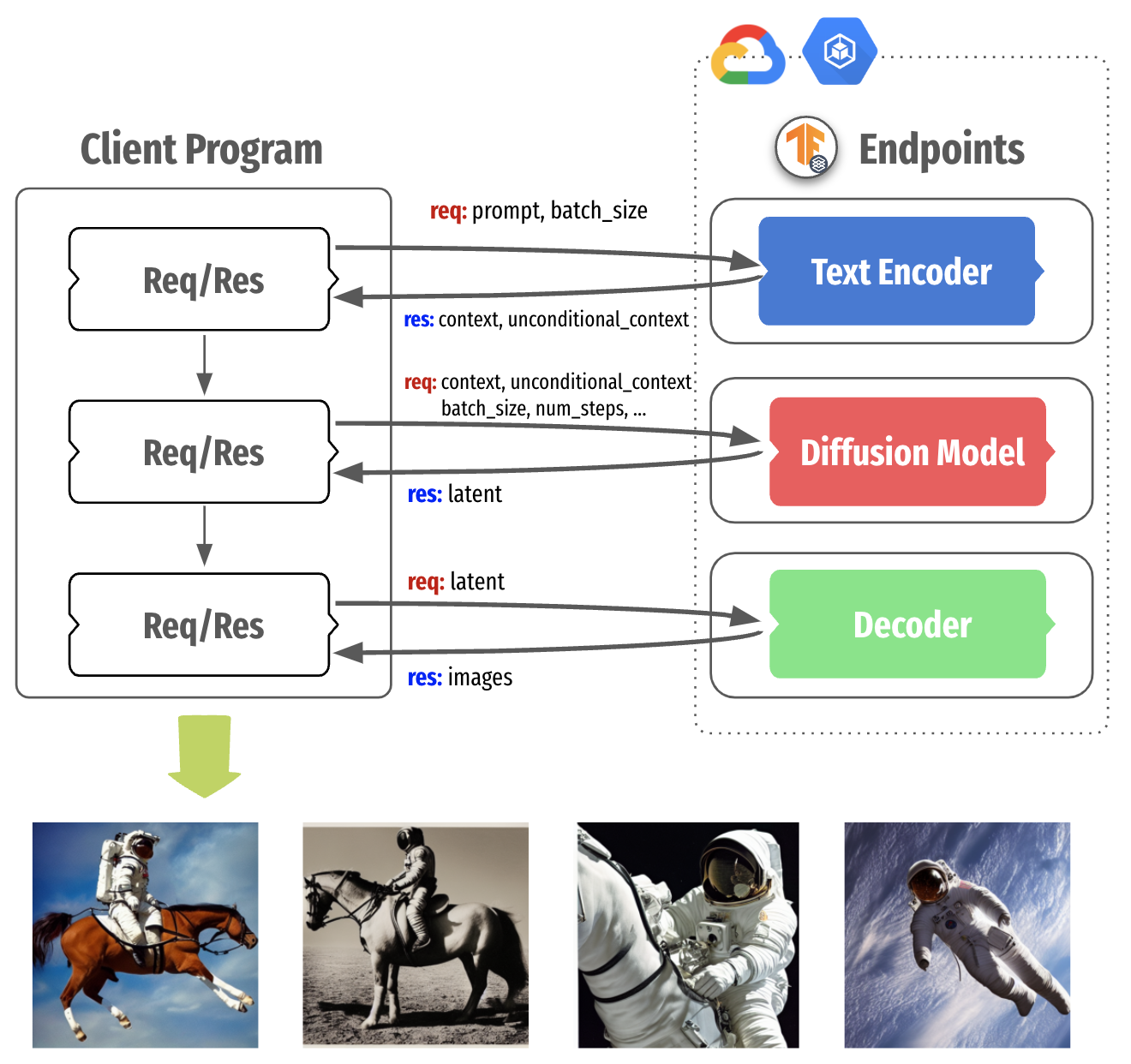
Once all the TensorFlow Serving instances are deployed, we could generate images by calling their endpoints. We will show how to do it through RestAPI, but you could do the same with the gRPC channel as well. The image generation process could be done in the following steps:
- Prepare tokens for the prompt of your choice
- Send the tokens to the Text Encoder endpoint
- Send context and unconditional context obtained from the Text Encoder to the Diffusion Model endpoint
- Send latent obtained from the Diffusion Model to the Decoder endpoint
- Plot the generated images
Since it is non-trivial to embed a tokenizer into the Text Encoder itself, we need to prepare the tokens for the prompt of your choice. KerasCV library provides SimpleTokenizer in the keras_cv.models.stable_diffusion.clip_tokenizer module, so you could simply pass the prompt to it. Since the Diffusion Model is designed to accept 77 tokens, the tokens are padded with MAX_PROMPT_LENGTH up to 77 long.
NOTE: Since KerasCV comes with lots of modules that we don’t need for tokenization, it is not recommended to import the entire library. Instead, you could simply copy the codes for the SimpleTokenizer in your environment. Due to incompatibility issues, the current tokenizer cannot be shipped as a part of the Text Encoder SavedModel.
from keras_cv.models.stable_diffusion.clip_tokenizer import SimpleTokenizer

MAX_PROMPT_LENGTH = 77
PADDING_TOKEN = 49407

tokenizer = SimpleTokenizer()

prompt = "photograph of an astronaut riding a horse in a green desert"
tokens = tokenizer.encode(prompt)
tokens = tokens + [PADDING_TOKEN] * (MAX_PROMPT_LENGTH - len(tokens)) |
Once the tokens are prepared, we could simply pass it to the Diffusion Model’s endpoint. The headers and the way to call the all endpoints are identical as below, so we will omit it in the following steps. Just keep in mind you set the ADDRESS and the MODEL_NAME correctly, which is identical to the one we set in each Dockerfile.
import requests

ADDRESS = ENDPOINT_IP_ADDRESS

headers = {"content-type": "application/json"}
payload = ENDPOINT_SPECIFIC

response = requests.post(
    f"http://{ADDRESS}:8501/v1/models/{MODEL_NAME}:predict",
    data=payload, headers=headers
) |
As you see, each payload is dependent on the upstream tasks. For instance, we pass tokens to the Text Encoder’s endpoint, context and unconditional_context retrieved from the Text Encoder to the Diffusion Model’s endpoint, and latent retrieved from the Diffusion Model to Decoder’s endpoint. The signature_name should be the same as when we created SavedModel with the signatures argument.
import json


BATCH_SIZE = 4

payload_to_text_encoder = json.dumps(
    {
        "signature_name": "serving_default",
        "inputs": {
            "tokens": tokens,
            "batch_size": BATCH_SIZE
        }
})

# json_response is from the text_encoder's response
# json_response = json.loads(response.text)
payload_to_diffusion_model = json.dumps(
    {
        "signature_name": "serving_default",
        "inputs": {
            "batch_size": BATCH_SIZE,
            "context": json_response['outputs']['context'],
            "num_steps": num_steps,
            "unconditional_context": json_response['outputs']['unconditional_context']
        }
})

# json_response is from the diffusion_model's response
# json_response = json.loads(response.text)
payload_to_decoder = json.dumps(
    {
        "signature_name": "serving_default",
        "inputs": {
            "latent": json_response['outputs'],
        }
}) |
The final response from the Decoder’s endpoint contains a full of pixel values in a list, so we need to convert those into a format that the environment of your choice could understand as images. For demonstration purposes, we used the tf.convert_to_tensor() utility function that turns the Python list into TensorFlow’s Tensor. However, you could plot the images in different languages, too, with your most familiar methods.
import matplotlib.pyplot as plt

def plot_images(images):
    plt.figure(figsize=(20, 20))
    for i in range(len(images)):
        ax = plt.subplot(1, len(images), i + 1)
        plt.imshow(images[i])
        plt.axis("off")

plot_images(
    tf.convert_to_tensor(json_response['outputs']).numpy()
) |
 |
| Figure 4. Generated images with three TensorFlow Serving endpoints |
We can obtain a speed-up of 17 - 25% by incorporating compiling the SavedModels to be XLA compatible. Note that the individual sub-networks of the Stable Diffusion class are fully XLA compatible. But in our case, the SavedModels also contain important operations that are in native TensorFlow, such as the reverse diffusion process.
For deployment purposes, this speed-up could be impactful. To know more, check out the following repository: https://github.com/sayakpaul/xla-benchmark-sd.
In this blog post, we explored what Stable Diffusion is, how it could be decomposed into the Text Encoder, Diffusion Model, and Decoder, and why it might be beneficial for better resource utilization. Also, we touched upon the concrete demonstration about the deployment of the decomposed Stable Diffusion by creating SavedModels, containerizing them in TensorFlow Serving, deploying them on the GKE cluster, and running image generations. We used the vanilla Stable Diffusion, but feel free to try out replacing the only Diffusion Model with in-painting or pokemon fine-tuned diffusion models.
CLIP: Connecting text and images, OpenAI, https://openai.com/research/clip.
The Illustrated Stable Diffusion, Jay Alammar, https://jalammar.github.io/illustrated-stable-diffusion/.
Stable Diffusion, Stability AI, https://stability.ai/stable-diffusion.
We are grateful to the ML Developer Programs team that provided Google Cloud credits to support our experiments. We thank Robert Crowe for providing us with helpful feedback and guidance.
___________
1 Stable Diffusion is not owned or operated by Google. It is made available by Stability AI. Please see their site for more information: https://stability.ai/blog/stable-diffusion-public-release.

dubna 28, 2023 — Posted by Chansung Park and Sayak Paul (ML and Cloud GDEs)Generative AI models like Stable Diffusion1 that lets anyone generate high-quality images from natural language text prompts enable different use cases across different industries. These types of models allow people to generate these images not only from images but also condition them with other inputs such as segmentation maps, other imag…


