
Modern recommenders heavily leverage embeddings to create vector representations of each user and candidate item. These embedding can then be used to calculate the similarity between users and items, so that users are recommended candidate items that are more interesting and relevant. But when working with data at scale, particularly in an online machine learning setting, embedding tables can grow in size dramatically, accumulating millions (and sometimes billions) of items. At this scale, it becomes impossible to store these embedding tables in memory. Furthermore, a large portion of the items might be rarely seen, so it does not make sense to keep dedicated embeddings for such rarely occurring items. A better solution would be to represent those items with one common embedding. This can dramatically reduce the size of the embedding table at a very small fraction of the performance cost. This is the main motivation behind dynamic embedding tables.
TensorFlow's built-in tf.keras.layers.Embedding layer has a fixed size at creation time, so we need another approach. Fortunately, there is a TensorFlow SIG project exactly for this purpose: TensorFlow Recommenders Addons (TFRA). You can learn more from its repository, but at a high level TFRA leverages dynamic embedding technology to dynamically change embedding size and achieve better recommendation results than static embeddings. TFRA is fully TF2.0-compatible and works smoothly with the familiar Keras API interfaces, so it can be easily integrated with other TensorFlow products, such as TensorFlow Recommenders (TFRS).
In this tutorial we will build a movie recommender model by leveraging both TFRS and TFRA. We will use the MovieLens dataset, which contains anonymized data showing ratings given to movies by users. Our primary focus is to show how the dynamic embeddings provided in the TensorFlow Recommenders Addons library can be used to dynamically grow and shrink the size of the embedding tables in the recommendation setting. You can find the full implementation here and a walkthrough here.
We will first import the required libraries.
import tensorflow as tf
import tensorflow_datasets as tfds

#TFRA does some patching on TensorFlow so it MUST be imported after importing TF
import tensorflow_recommenders as tfrs
import tensorflow_recommenders_addons as tfra
import tensorflow_recommenders_addons.dynamic_embedding as de |
Note how we are importing the TFRA library after importing TensorFlow. It is recommended to follow this ordering as the TFRA library will be applying some patches on TensorFlow.
Let’s first build a baseline model with TensorFlow Recommenders. We will follow the pattern of this TFRS retrieval tutorial to build a two-tower retrieval model. The user tower will take the user ID as the input, but the item tower will use the tokenized movie title as the input.
To handle the movie titles, we define a helper function that converts the movie titles to lowercase, removes any punctuation in a given movie title, and splits using spaces to generate a list of tokens. Finally we take only the up to max_token_length tokens (from the start) from the movie title. If a movie title has fewer tokens, all the tokens will be taken. This number is chosen based on some analysis and represents the 90th percentile in the title lengths in the dataset.
max_token_length = 6
pad_token = "[PAD]"
punctuation_regex = "[\!\"#\$%&\(\)\*\+,-\.\/\:;\<\=\>\?@\[\]\\\^_`\{\|\}~\\t\\n]"

#First we’ll define a helper function that will process the movie titles for us.

def process_text(x: tf.Tensor, max_token_length: int, punctuation_regex: str) -> tf.Tensor:

	return tf.strings.split(
    		tf.strings.regex_replace(
        			tf.strings.lower(x["movie_title"]), punctuation_regex, ""
    		)
)[:max_token_length] |
We also pad the tokenized movie titles to a fixed length and split the dataset using the same random seed so that we get consistent validation results across training epochs. You can find detailed code in the ‘Processing datasets’ section of the notebook.
Our user tower is pretty much the same as in the TFRS retrieval tutorial (except it’s deeper), but for the movie tower there is a GlobalAveragePooling1D layer after the embedding lookup, which averages the embedding of movie title tokens to a single embedding.
def get_movie_title_lookup_layer(dataset: tf.data.Dataset) -> tf.keras.layers.Layer:
	movie_title_lookup_layer = tf.keras.layers.StringLookup(mask_token=pad_token)
	movie_title_lookup_layer.adapt(dataset.map(lambda x: x["movie_title"]))
	return movie_title_lookup_layer

def build_item_model(movie_title_lookup_layer: tf.keras.layers.StringLookup):
	vocab_size = movie_title_lookup_layer.vocabulary_size()
	return tf.keras.models.Sequential([
    	tf.keras.layers.InputLayer(input_shape=(max_token_length), dtype=tf.string),
    	movie_title_lookup_layer,
    	tf.keras.layers.Embedding(vocab_size, 64),
    	tf.keras.layers.GlobalAveragePooling1D(),
    	tf.keras.layers.Dense(64, activation="gelu"),
    	tf.keras.layers.Dense(32),
    	tf.keras.layers.Lambda(lambda x: tf.math.l2_normalize(x, axis=1))
]) |
Next we are going to train the model.
Training the model is simply calling fit() on the model with the required arguments. We will be using our validation dataset validation_ds to measure the performance of our model.
history = model.fit(datasets.training_datasets.train_ds, epochs=3, validation_data=datasets.training_datasets.validation_ds) |
At the end, the output looks like below:
Epoch 3/3
220/220 [==============================] - 146s 633ms/step
......
val_factorized_top_k/top_10_categorical_accuracy: 0.0179 - val_factorized_top_k/top_50_categorical_accuracy: 0.0766 - val_factorized_top_k/top_100_categorical_accuracy: 0.1338 - val_loss: 12359.0557 - val_regularization_loss: 0.0000e+00 - val_total_loss: 12359.0557 |
We have achieved a top 100 categorical accuracy of 13.38% on the validation dataset.
We will now learn how we can use the dynamic embedding in the TensorFlow Recommenders Addons (TFRA) library, rather than a static embedding table. As the name suggests, as opposed to creating embeddings for all the items in the vocabulary up front, dynamic embedding would only grow the size of the embedding table on demand. This behavior really shines when dealing with millions and billions of items and users as some companies do. For these companies, it’s not surprising to find static embedding tables that would not fit in memory. Static embedding tables can grow up to hundreds of Gigabytes or even Terabytes, incapacitating even the highest memory instances available in cloud environments.
When you have an embedding table with large cardinality, the accessing weights will be quite sparse. Therefore, a hash-table based data structure is used to hold the weights and required weights for each iteration are retrieved from the underlying table structure. Here, to focus on the core functionality of the library, we will focus on a non-distributed setting. In this case, TFRA will choose cuckoo hashtable by default. But there are other solutions such as Redis, nvhash available.
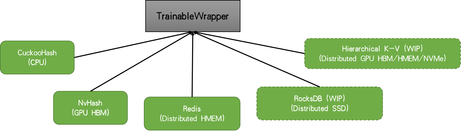 |
When using the dynamic embedding, we initialize the table with some initial capacity and the table will grow in size on demand as it sees more IDs during model training. For more information about motivation and inner mechanics, please refer to the RFC.
Currently in the TFRA dynamic_embedding module, there are three types of embedding available:
n_slots as an argument and IDs are mapped to a slot within the layer. The layer would return a tensor of size [batch_size, n_slots, embedding_dim]. We will be using the Embedding to represent the user IDs and SquashedEmbedding to represent token IDs. Remember that each movie title has multiple tokens, therefore, we need a way to reduce the resulting token embeddings to a single representative embedding.
Note: The behavior of Embedding has changed from version 0.5 to 0.6. Please make sure to use version 0.6 for this tutorial.
With that, we can define the two towers as we did in the standard model. However, this time we’ll be using the dynamic embedding layers instead of static embedding layers.
def build_de_user_model(user_id_lookup_layer: tf.keras.layers.StringLookup) -> tf.keras.layers.Layer:
	vocab_size = user_id_lookup_layer.vocabulary_size()
	return tf.keras.Sequential([
    	tf.keras.layers.InputLayer(input_shape=(), dtype=tf.string),
    	user_id_lookup_layer,
    	de.keras.layers.Embedding(
        	embedding_size=64,
        	initializer=tf.random_uniform_initializer(),
        	init_capacity=int(vocab_size*0.8),
        	restrict_policy=de.FrequencyRestrictPolicy,
        	name="UserDynamicEmbeddingLayer"
    	),
    	tf.keras.layers.Dense(64, activation="gelu"),
    	tf.keras.layers.Dense(32),
    	tf.keras.layers.Lambda(lambda x: tf.math.l2_normalize(x, axis=1))
	], name='user_model')

def build_de_item_model(movie_title_lookup_layer: tf.keras.layers.StringLookup) -> tf.keras.layers.Layer:
	vocab_size = movie_title_lookup_layer.vocabulary_size()
	return tf.keras.models.Sequential([
    		tf.keras.layers.InputLayer(input_shape=(max_token_length), dtype=tf.string),
    	movie_title_lookup_layer,
    	de.keras.layers.SquashedEmbedding(
        	embedding_size=64,
        	initializer=tf.random_uniform_initializer(),
        	init_capacity=int(vocab_size*0.8),
        	restrict_policy=de.FrequencyRestrictPolicy,
        	combiner="mean",
        	name="ItemDynamicEmbeddingLayer"
    	),
    	tf.keras.layers.Dense(64, activation="gelu"),
    	tf.keras.layers.Dense(32),
    	tf.keras.layers.Lambda(lambda x: tf.math.l2_normalize(x, axis=1))
]) |
With the user tower and movie tower models defined, we can define the retrieval model as usual.
As a final step in model building, we’ll create the model and compile it.
def create_de_two_tower_model(dataset: tf.data.Dataset, candidate_dataset: tf.data.Dataset) -> tf.keras.Model:

	user_id_lookup_layer = get_user_id_lookup_layer(dataset)
	movie_title_lookup_layer = get_movie_title_lookup_layer(dataset)
	user_model = build_de_user_model(user_id_lookup_layer)
	item_model = build_de_item_model(movie_title_lookup_layer)
	task = tfrs.tasks.Retrieval(
    	metrics=tfrs.metrics.FactorizedTopK(
        	candidate_dataset.map(item_model)
    	),
	)

	model = DynamicEmbeddingTwoTowerModel(user_model, item_model, task)
	optimizer = de.DynamicEmbeddingOptimizer(tf.keras.optimizers.Adam())
	model.compile(optimizer=optimizer)

	return model

datasets = create_datasets()
de_model = create_de_two_tower_model(datasets.training_datasets.train_ds, datasets.candidate_dataset) |
Note the usage of the DynamicEmbeddingOptimizer wrapper around the standard TensorFlow optimizer. It is mandatory to wrap the standard optimizer in a DynamicEmbeddingOpitmizer as it will provide specialized functionality needed to train the weights stored in a hashtable. We can now train our model.
Training the model is quite straightforward, but will involve a bit more extra effort as we’d like to log some extra information. We will perform the logging through a tf.keras.callbacks.Callback object. We’ll name this DynamicEmbeddingCallback.
epochs = 3
history_de = {}
history_de_size = {}
de_callback = DynamicEmbeddingCallback(de_model, steps_per_logging=20)

for epoch in range(epochs):

	datasets = create_datasets()
	train_steps = len(datasets.training_datasets.train_ds)

	hist = de_model.fit(
    	datasets.training_datasets.train_ds,
    	epochs=1,
    	validation_data=datasets.training_datasets.validation_ds,
    	callbacks=[de_callback]
	)

	for k,v in de_model.dynamic_embedding_history.items():
    	if k=="step":
        		v = [vv+(epoch*train_steps) for vv in v]
    	history_de_size.setdefault(k, []).extend(v)

	for k,v in hist.history.items():
history_de.setdefault(k, []).extend(v) |
We have taken the loop that goes through the epochs out of the fit() function. Then in every epoch we re-create the dataset, as that will provide a different shuffling of the training dataset. We will train the model for a single epoch within the loop. Finally we accumulate the logged embedding sizes in history_de_size (this is provided by our custom callback) and performance metrics in history_de.
The callback is implemented as follows.
class DynamicEmbeddingCallback(tf.keras.callbacks.Callback):

    def __init__(self, model, steps_per_logging, steps_per_restrict=None, restrict=False):
        self.model = model
        self.steps_per_logging = steps_per_logging
        self.steps_per_restrict = steps_per_restrict
        self.restrict = restrict

    def on_train_begin(self, logs=None):
        self.model.dynamic_embedding_history = {}

    def on_train_batch_end(self, batch, logs=None):

        if self.restrict and self.steps_per_restrict and (batch+1) % self.steps_per_restrict == 0:

            [
                self.model.embedding_layers[k].params.restrict(
                    num_reserved=int(self.model.lookup_vocab_sizes[k]*0.8),
                    trigger=self.model.lookup_vocab_sizes[k]-2 # UNK & PAD tokens
                ) for k in self.model.embedding_layers.keys()
            ]

        if (batch+1) % self.steps_per_logging == 0:

            embedding_size_dict = {
                k:self.model.embedding_layers[k].params.size().numpy()
                for k in self.model.embedding_layers.keys()
            }

            for k, v in embedding_size_dict.items():
                self.model.dynamic_embedding_history.setdefault(f"embedding_size_{k}", []).append(v)
self.model.dynamic_embedding_history.setdefault(f"step", []).append(batch+1) |
The callback does two things:
steps_per_logging iterationsrestrict=True(This is set to False by default)Let’s understand what reducing the size means and why it is important.
An important topic we still haven’t discussed is how to reduce the size of the embedding table, should it grow over some predefined threshold. This is a powerful functionality as it allows us to define a threshold over which the embedding table should not grow. This will allow us to work with large vocabularies while keeping the memory requirement under the memory limitations we may have. We achieve this by calling restrict() on the underlying variables of the embedding layer as shown in the DynamicEmbeddingCallback. restrict() takes two arguments in: num_reserved (the size after the reduction) and trigger (size at which the reduction should be triggered). The policy that governs how the reduction is performed is defined using the restrict_policy argument in the layer construct. You can see that we are using the FrequencyRestrictPolicy. This means the least frequent items will be removed from the embedding table. The callback enables a user to set how frequently the reduction should get triggered by setting the steps_per_restrict and restrict arguments in the DynamicEmbeddingCallback.
Reducing the size of the embedding table makes more sense when you have streaming data. Think about an online learning setting, where you are training the model every day (or even every hour) on some incoming data. You can think of the outer for loop (i.e. epochs) representing days. Each day you receive a dataset (containing user interactions from the previous day for example) and you train the model from the previous checkpoint. In this case, you can use the DynamicEmbeddingCallback to trigger a restrict if the embedding table grows over the size defined in the trigger argument.
Here we analyze the performance of three variants.
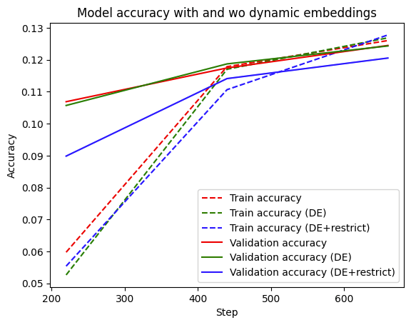 |
You can see that the model using dynamic embeddings (solid green line) has comparative validation performance to the baseline (solid red line). You can see a similar trend in the training accuracy as well. In practice, dynamic embeddings can often be seen to improve accuracy in a large-scale online learning setup.
Finally, we can see that restrict has a somewhat detrimental effect on the validation accuracy, which is understandable. Since we’re working with a relatively small dataset with a small number of items, the reduction could be getting rid of embeddings that are best kept in the table. For example, you can increase the num_reserved argument (e.g. set it to int(self.model.lookup_vocab_sizes[k]*0.95)) in the restrict function which would yield performance that improves towards the performance of without restrict.
Next we look at how dynamic the embedding tables really are over time.
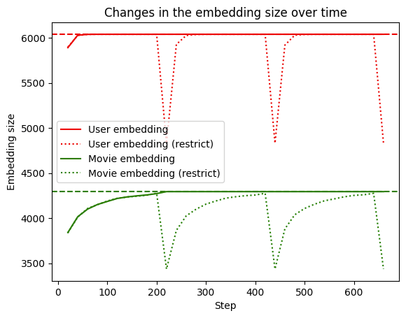 |
We can see that when restrict is not used, the embedding table grows to the full size of the vocabulary (dashed line) and stays there. However when restrict is triggered (dotted line), the size drops and grows in size again as it encounters new IDs.
It is also important to note that constructing a proper validation is not a trivial task. There are considerations such as out-of-sample validation, out-of-time validation, stratification, etc. that needs to be taken into account carefully. However for this exercise, we have not focused on such factors and created a validation set by sampling randomly from the existing dataset.
Using dynamic embedding tables is a powerful way to perform representation learning when working with large sets of items containing millions or billions of entities. In this tutorial, we learnt how to use the dynamic_embedding module provided in the TensorFlow Recommender Addons library to achieve this. We first explored the data and constructed tf.data.Dataset objects by extracting the features we’ll be using for our model training and evaluation. Next we defined a model that uses static embedding tables to use as an evaluation baseline. We then created a model that uses dynamic embedding and trained it on the data. We saw that using dynamic embeddings, the embedding tables grow only on demand and still achieve comparable performance with the baseline. We also discussed how the restrict functionality can be used to shrink the embedding table if it grows past a pre-defined threshold.
We hope this tutorial gives you a good conceptual introduction to TFRA and dynamic embeddings, and helps you think about how you can leverage it to enhance your own recommenders. If you would like to have a more in-depth discussion, please visit the TFRA repository.


aprile 19, 2023 — Posted by Thushan Ganegedara (GDE), Haidong Rong (Nvidia), Wei Wei (Google)Modern recommenders heavily leverage embeddings to create vector representations of each user and candidate item. These embedding can then be used to calculate the similarity between users and items, so that users are recommended candidate items that are more interesting and relevant. But when working with data at scale, p…


