de maig 02, 2023 — Posted by Jeremy Wortz, ML specialist, Google Cloud & Jordan Totten, Machine Learning Specialist Cross posted from Google Cloud AI & Machine LearningIn a previous blog, we outlined three approaches for implementing recommendation systems on Google Cloud, including (1) a fully managed solution with Recommendations AI, (2) matrix factorization from BigQuery ML, and (3) custom deep retrieval…

Posted by Jeremy Wortz, ML specialist, Google Cloud & Jordan Totten, Machine Learning Specialist
Cross posted from Google Cloud AI & Machine Learning
In a previous blog, we outlined three approaches for implementing recommendation systems on Google Cloud, including (1) a fully managed solution with Recommendations AI, (2) matrix factorization from BigQuery ML, and (3) custom deep retrieval techniques using two-tower encoders and Vertex AI Matching Engine. In this blog, we dive deep into option (3) and demonstrate how to build a playlist recommendation system by implementing an end-to-end candidate retrieval workflow from scratch with Vertex AI. Specifically, we will cover:
- The evolution of retrieval modeling and why two-tower encoders are popular for deep retrieval tasks
- Framing a playlist-continuation use-case using the Spotify Million Playlist Dataset (MPD)
- Developing custom two-tower encoders with the TensorFlow Recommenders (TFRS) library
- Serving candidate embeddings in an approximate nearest neighbors (ANN) index with Vertex AI Matching Engine
All related code can be found in this GitHub repository.
To meet low latency serving requirements, large-scale recommenders are often deployed to production as multi-stage systems. The goal of the first stage (candidate retrieval) is to sift through a large (>100M elements) corpus of candidate items and retrieve a relevant subset (~hundreds) of items for downstream ranking and filtering tasks. To optimize this retrieval task, we consider two core objectives:
- During model training, find the best way to compile all knowledge into
query, candidateembeddings.- During model serving, retrieve relevant items fast enough to meet latency requirements
 |
| Figure 1: Conceptual components of multi-stage recommendation systems; the focus of this blog is the first stage, candidate retrieval. |
Two-tower architectures are popular for retrieval tasks because they capture the semantics of query and candidate entities, and map these to a shared embedding space such that semantically similar entities cluster closer together. This means, if we compute the vector embeddings of a given query, we can search the embedding space for the closest (most similar) candidates. Because these neural network-based retrieval models take advantage of metadata, context, and feature interactions, they can produce highly informative embeddings and offer flexibility to adjust for various business objectives.
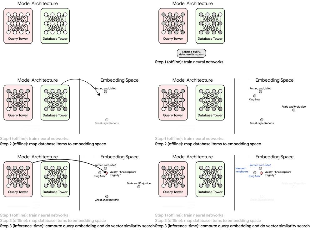 |
| Figure 2: The two-tower encoder model is a specific type of embedding-based search where one deep neural network tower produces the query embedding and a second tower computes the candidate embedding. Calculating the dot product between the two embedding vectors determines how close (similar) the candidate is to the query. Source: Announcing ScaNN: Efficient Vector Similarity Search. |
While these capabilities help achieve useful query, candidate embeddings, we still need to resolve the retrieval latency requirements. To this end, the two-tower architecture offers one more advantage: the ability to decouple inference of query and candidate items. This decoupling means all candidate item embeddings can be precomputed, reducing the serving computation to (1) converting queries to embedding vectors and (2) searching for similar vectors (among the precomputed candidates).
As candidate datasets scale to millions (or billions) of vectors, the similarity search often becomes a computational bottleneck for model serving. Relaxing the search to approximate distance calculations can lead to significant latency improvements, but we need to minimize negatively impacting search accuracy (i.e., relevance, recall).
In the paper Accelerating Large-Scale Inference with Anisotropic Vector Quantization, Google Researchers address this speed-accuracy tradeoff with a novel compression algorithm that, compared to previous state-of-the-art methods, improves both the relevance and speed of retrieval. At Google, this technique is widely-adopted to support deep retrieval use cases across Search, YouTube, Ads, Lens, and others. And while it’s available in an open-sourced library (ScaNN), it can still be challenging to implement, tune, and scale. To help teams take advantage of this technology without the operational overhead, Google Cloud offers these capabilities (and more) as a managed service with Vertex AI Matching Engine.
The goal of this post is to demonstrate how to implement these deep retrieval techniques using Vertex AI and discuss the decisions and trade-offs teams will need to evaluate for their use cases.
 |
| Figure 3: Figure 3: A reference architecture for two-tower training and deployment on Vertex AI. |
To better understand the benefits of two-tower architectures, let’s review three key modeling milestones in candidate retrieval.
Traditional information retrieval systems rely heavily on token-based matching, where candidates are retrieved using an inverted index of n-grams. These systems are interpretable, easy to maintain (e.g., no training data), and are capable of achieving high precision. However, they typically suffer poor recall (i.e., trouble finding all relevant candidates for a given query) because they look for candidates having exact matches of key words. While they are still used for select Search use cases, many retrieval tasks today are either adapted with or replaced by embedding-based techniques.
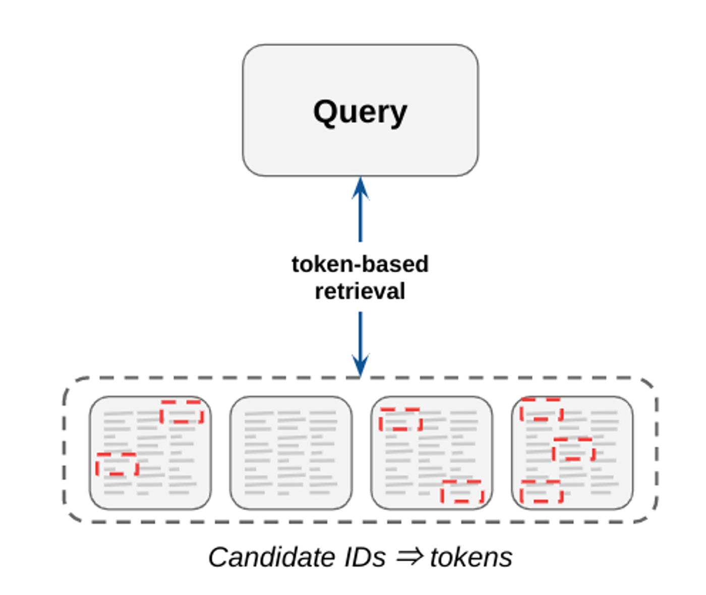 |
| Figure 4: Token-based matching selects candidate items by matching key words found in both query and candidate items. |
Factorization-based retrieval introduces a simple embedding-based model that offers much better generalization by capturing the similarity between query, candidate pairs and mapping them to a shared embedding space. One of the major benefits to this collaborative filtering technique is that embeddings are learned automatically from implicit query-candidate interactions. Fundamentally, these models factorize the full query-candidate interaction (co-occurrence) matrix to produce smaller, dense embedding representations of queries and candidates, where the product of these embedding vectors is a good approximation of the interaction matrix. The idea is that by compacting the full matrix into k dimensions the model learns the top k latent factors describing query, candidate pairs with respect to the modeling task.
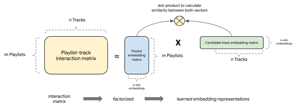 |
| Figure 5: Factorization-based models factorize a query-candidate interaction matrix into the product of two lower-rank matrices that capture the query-candidate interactions. |
The latest modeling paradigm for retrieval, commonly referred to as neural deep retrieval (NDR), produces the same embedding representations, but uses deep learning to create them. NDR models like two-tower encoders apply deep learning by processing input features with successive network layers to learn layered representations of the data. Effectively, this results in a neural network that acts as an information distillation pipeline, where raw, multi-modal features are repeatedly transformed such that useful information is magnified and irrelevant information is filtered. This results in a highly expressive model capable of learning non-linear relationships and more complex feature interactions.
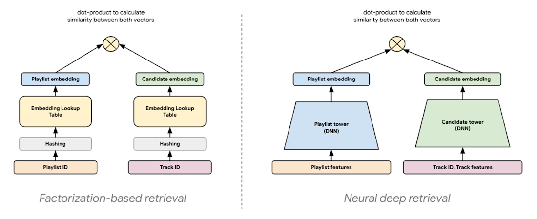 |
| Figure 6: NDR architectures like two-tower encoders are conceptually similar to factorization models. Both are embedding-based retrieval techniques computing lower-dimensional vector representations of query and candidates, where the similarity between these two vectors is determined by computing their dot product. |
In a two-tower architecture, each tower is a neural network that processes either query or candidate input features to produce an embedding representation of those features. Because the embedding representations are simply vectors of the same length, we can compute the dot product between these two vectors to determine how close they are. This means the orientation of the embedding space is determined by the dot product of each query, candidate pair in the training examples.
In addition to increased expressivity and generalization, this kind of architecture offers optimization opportunities for serving. Because each tower only uses its respective input features to produce a vector, the trained towers can be operationalized separately. Decoupling inference of the towers for retrieval means we can precompute what we want to find when we encounter its pair in the wild. It also means we can optimize each inference task differently:
- Run a batch prediction job with a trained candidate tower to precompute embedding vectors for all candidates, attach NVIDIA GPU to accelerate computation
- Compress precomputed candidate embeddings to an ANN index optimized for low-latency retrieval; deploy index to an endpoint for serving
- Deploy trained query tower to an endpoint for converting queries to embeddings in real time, attach NVIDIA GPU to accelerate computation
Training two-tower models and serving them with an ANN index is different from training and serving traditional machine learning (ML) models. To make this clear, let’s review the key steps to operationalize this technique.
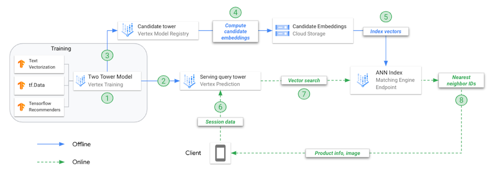 |
| Figure 7: A reference architecture for two-tower training and deployment on Vertex AI. |
- Train combined model (two-towers) offline; each tower is saved separately for different tasks
- Upload the query tower to Vertex AI Model Registry and deploy to an online endpoint
- Upload the candidate tower to Vertex AI Model Registry
- Request candidate tower to predict embeddings for each candidate track, save embeddings in JSON file
- Create ANN serving index from embeddings JSON, deploy to online index endpoint
- User application calls endpoint.predict() with playlist data, model returns the embedding vector representing that playlist
- Use the playlist embedding vector to search for N nearest neighbors (candidate tracks)
- Matching Engine returns the product IDs for the N nearest neighbors
In this example, we use MPD to construct a recommendation use case, playlist continuation, where candidate tracks are recommended for a given playlist (query). This dataset is publicly available and offers several benefits for this demonstration:
- Includes real relationships between entities (e.g., playlists, tracks, artists) which can be difficult to replicate
- Large enough to replicate scalability issues likely to occur in production
- Variety of feature representations and data types (e.g., playlist and track IDs, raw text, numerical, datetime); ability to enrich dataset with additional metadata from the Spotify Web Developer API
- Teams can analyze the impact of modeling decisions by listening to retrieved candidate tracks (e.g., generate recommendations for your own Spotify playlists)
Creating training examples for recommendation systems is a non-trivial task. Like any ML use case, training data should accurately represent the underlying problem we are trying to solve. Failure to do this can lead to poor model performance and unintended consequences for the user experience. One such lesson from the Deep Neural Networks for YouTube Recommendations paper highlights that relying heavily on features such as ‘click-through rate’ can result in recommending clickbait (i.e., videos users rarely complete), as compared to features like ‘watch time’ which better capture a user’s engagement.
Training examples should represent a semantic match in the data. For playlist-continuation, we can think of a semantic match as pairing playlists (i.e., a set of tracks, metadata, etc.) with tracks similar enough to keep the user engaged with their listening session. How does the structure of our training examples influence this?
- Training data is sourced from positive
query, candidatepairs- During training, we forward propagate query and candidate features through their respective towers to produce the two vector representations, from which we compute the dot product representing their similarity
- After training, and before serving, the candidate tower is called to predict (precompute) embeddings for all candidate items
- At serving time, the model processes features for a given playlist and produces a vector embedding
- The playlist’s vector embedding is used in a search to find the most similar vectors in the precomputed candidate index
- The placement of candidate and playlist vectors in the embedding space, and the distance between them, is defined by the semantic relationships reflected in the training examples
The last point is important. Because the quality of our embedding space dictates the success of our retrieval, the model creating this embedding space needs to learn from training examples that best illustrate the relationship between a given playlist and similar tracks to retrieve.
This notion of similarity being highly dependent on the choice of paired data highlights the importance of preparing features that describe semantic matches. A model trained on playlist title, track title pairs will orient candidate tracks differently than a model trained on aggregated playlist audio features, track audio features pairs.
Conceptually, training examples consisting of playlist title, track title pairs would create an embedding space in which all tracks belonging to playlists of the same or similar titles (e.g., beach vibes and beach tunes) would be closer together than tracks belonging to different playlist titles (e.g., beach vibes vs workout tunes); and examples consisting of aggregated playlist audio features, track audio features pairs would create an embedding space in which all tracks belonging to playlists with similar audio profiles (e.g., live recordings of instrumental jams and high energy instrumentals) would be closer together than tracks belonging to playlists with different audio profiles (e.g., live recordings of instrumental jams vs acoustic tracks with lots of lyrics).
The intuition for these examples is that when we structure the rich track-playlist features in a format that describes how tracks show up on certain playlists, we can feed this data to a two tower model that learns all of the niche relationships between parent playlist and child tracks. Modern deep retrieval systems often consider user profiles, historical engagements, and context. While we don’t have user and context data in this example, they can easily be added to the query tower.
When building retrieval models with TFRS, the two towers are implemented with model subclassing. Each tower is built separately as a callable to process input feature values, pass them through feature layers, and concatenate the results. This means the tower is simply producing one concatenated vector (i.e., the representation of the query or candidate; whatever the tower represents). First, we define the basic structure of a tower and implement it as a subclassed Keras model:
class Playlist_Tower(tf.keras.Model):
   '''
   produced embedding represents the features
   of a Playlist known at query time
   '''
   def __init__(self, layer_sizes, vocab_dict):
       super().__init__()

       # TODO: build sequential model for each feature here

   def call(self, data):
       '''
       defines what happens when the model is called
       '''
       all_embs = tf.concat(
           [
               # TODO: concatenate output of all features defined above

           ], axis=1)

       # pass output to dense/cross layers
       if self._cross_layer is not None:
           cross_embs = self._cross_layer(all_embs)
           return self.dense_layers(cross_embs)
       else:
return self.dense_layers(all_embs) |
We further define the subclassed towers by creating Keras sequential models for each feature being processed by that tower:
# Feature: pl_name_src
self.pl_name_src_text_embedding = tf.keras.Sequential(
   [
       tf.keras.layers.TextVectorization(
           vocabulary=vocab_dict['pl_name_src'],
           ngrams=2,
           name="pl_name_src_textvectorizor"
       ),
       tf.keras.layers.Embedding(
           input_dim=MAX_TOKENS,
           output_dim=EMBEDDING_DIM,
           name="pl_name_src_emb_layer",
           mask_zero=False
       ),
       tf.keras.layers.GlobalAveragePooling1D(name="pl_name_src_1d"),
   ], name="pl_name_src_text_embedding"
) |
Because the features represented in the playlist’s STRUCT are sequence features (lists), we need to reshape the embedding layer output and use 2D pooling (as opposed to the 1D pooling applied for non-sequence features):
# Feature: artist_genres_pl
self.artist_genres_pl_embedding = tf.keras.Sequential(
   [
       tf.keras.layers.TextVectorization(
           ngrams=2,
           vocabulary=vocab_dict['artist_genres_pl'],
           name="artist_genres_pl_textvectorizor"
       ),
       tf.keras.layers.Embedding(
           input_dim=MAX_TOKENS,
           output_dim=EMBED_DIM,
           name="artist_genres_pl_emb_layer",
           mask_zero=False
       ),
       tf.keras.layers.Reshape([-1, MAX_PL_LENGTH, EMBED_DIM]),
       tf.keras.layers.GlobalAveragePooling2D(name="artist_genres_pl_2d"),
   ], name="artist_genres_pl_emb_model"
) |
Once both towers are built, we use the TFRS base model class (tfrs.models.Model) to streamline building the combined model. We include each tower in the class __init__ and define the compute_loss method:
class TheTwoTowers(tfrs.models.Model):

   def __init__(self, layer_sizes, vocab_dict, parsed_candidate_dataset):
       super().__init__()

       self.query_tower = Playlist_Tower(layer_sizes, vocab_dict)

       self.candidate_tower = Candidate_Track_Tower(layer_sizes, vocab_dict)

       self.task = tfrs.tasks.Retrieval(
           metrics=tfrs.metrics.FactorizedTopK(
               candidates=parsed_candidate_dataset.batch(128).map(
                   self.candidate_tower,
                   num_parallel_calls=tf.data.AUTOTUNE
               ).prefetch(tf.data.AUTOTUNE)
           )
       )

   def compute_loss(self, data, training=False):

       query_embeddings = self.query_tower(data)
       candidate_embeddings = self.candidate_tower(data)

       return self.task(
           query_embeddings,
           candidate_embeddings,
           compute_metrics=not training,
           candidate_ids=data['track_uri_can'],
           compute_batch_metrics=True
) |
We can increase the depth of each tower by adding dense layers after the concatenated embedding layer. As this will emphasize learning successive layers of feature representations, this can improve the expressive power of our model.
Similarly, we can add deep and cross layers after our embedding layer to better model feature interactions. Cross layers model explicit feature interactions before combining with deep layers that model implicit feature interactions. These parameters often lead to better performance, but can significantly increase the computational complexity of the model. We recommend evaluating different deep and cross layer implementations (e.g., parallel vs stacked). See the TFRS Deep and Cross Networks guide for more details.
As the factorization-based models offer a pure collaborative filtering approach, the advanced feature processing with NDR architectures allow us to extend this to also incorporate aspects of content-based filtering. By including additional features describing playlists and tracks, we give NDR models the opportunity to learn semantic concepts about playlist, track pairs. The ability to include label features (i.e., features about candidate tracks) also means our trained candidate tower can compute an embedding vector for candidate tracks not observed during training (i.e., cold-start). Conceptually, we can think of such a new candidate track embedding compiling all the content-based and collaborative filtering information learned from candidate tracks with the same or similar feature values.
With this flexibility to add multi-modal features, we just need to process them to produce embedding vectors with the same dimensions so they can be concatenated and fed to subsequent deep and cross layers. This means if we use pre-trained embeddings as an input feature, we would pass these through to the concatenation layer (see Figure 8).
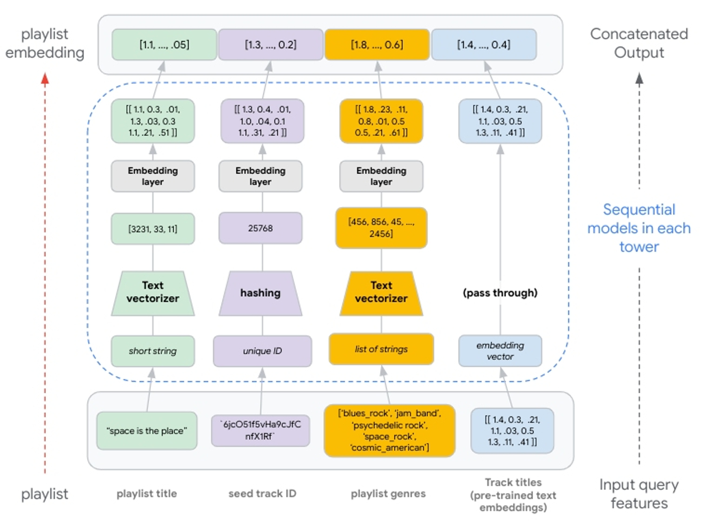 |
| Figure 8: Illustration of feature processing from input to concatenated output. Text features are generated via n-grams. Integer indexes of n-grams are passed to an embedding layer. Hashing produces unique integers up to 1,000,000; values passed to an embedding layer. If using pre-trained embeddings, these are passed through the tower without transformation and concatenated with the other embedding representations. |
Hashing is generally recommended when fast performance is needed and is preferred over string lookups because it skips the need for a lookup table. Setting the proper bin size for the hashing layer is critical. When there are more unique values than hashing bins, values start getting placed into the same bins, and this can negatively impact our recommendations. This is commonly referred to as a hashing collision, and can be avoided when building the model by allocating enough bins for the unique values. See turning categorical features into embeddings for more details.
The key to text features is to understand if creating additional NLP features with the TextVectorization layer is helpful. If additional context derived from the text feature is minimal, it may not be worth the cost to model training. This layer needs to be adapted from the source dataset, meaning the layer requires a scan of the training data to create lookup dictionaries for the top N n-grams (set by max_tokens).
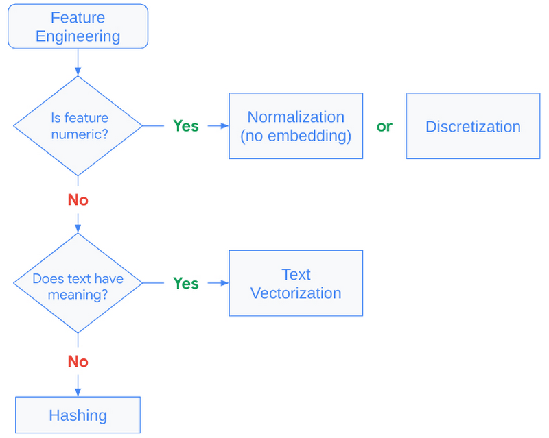 |
| Figure 9: Decision tree to guide feature engineering strategy. |
So far we’ve discussed how to map queries and candidates to the shared embedding space. Now let’s discuss how to best use this shared embedding space for efficient serving.
Recall at serving time, we will use the trained query tower to compute the embeddings for a query (playlist) and use this embedding vector in a nearest neighbor search for the most similar candidate (track) embeddings. And, because the candidate dataset can grow to millions or billions of vectors, this nearest neighbor search often becomes a computational bottleneck for low-latency inference.
Many state-of-the-art techniques address the computational bottleneck by compressing the candidate vectors such that ANN calculations can be performed in a fraction of the time needed for an exhaustive search. The novel compression algorithm proposed by Google Research modifies these techniques to also optimize for the nearest neighbor search accuracy. The details of their proposed technique are described here, but fundamentally their approach seeks to compress the candidate vectors such that the original distances between vectors are preserved. Compared to previous solutions, this results in a more accurate relative ranking of a vector and its nearest neighbors, i.e., it minimizes distorting the vector similarities our model learned from the training data.
Matching Engine is a managed solution utilizing these techniques for efficient vector similarity search. It offers customers a highly scalable vector database and ANN service while alleviating the operational overhead of developing and maintaining similar solutions, such as the open sourced ScaNN library. It includes several capabilities that simplify production deployments, including:
- Large-scale: supports large embedding datasets with up to 1 billion embedding vectors
- Incremental updates: depending on the number of vectors, complete index rebuilds can take hours. With incremental updates, customers can make small changes without building a new index (see Update and rebuild an active index for more details)
- Dynamic rebuilds: when an index grows beyond its original configuration, Matching Engine periodically re-organizes the index and serving structure to ensure optimal performance
- Autoscaling: underlying infrastructure is autoscaled to ensure consistent performance at scale
- Filtering and diversity: ability to include multiple restrict and crowding tags per vector. At query inference time, use boolean predicates to filter and diversify retrieved candidates (see Filter vector matches for more details)
When creating an ANN index, Matching Engine uses the Tree-AH strategy to build a distributed implementation of our candidate index. It combines two algorithms:
- Distributed search tree for hierarchically organizing the embedding space. Each level of this tree is a clustering of the nodes at the next level down, where the final leaf-level is a clustering of our candidate embedding vectors
- Asymmetric hashing (AH) for fast dot product approximation algorithm used to score similarity between a query vector and the search tree nodes
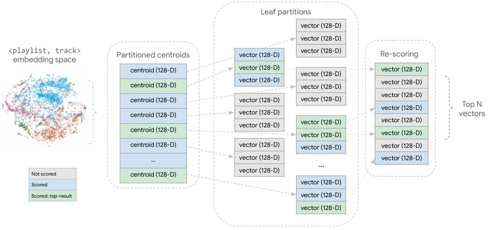 |
| Figure 10: conceptual representation of the partitioned candidate vector dataset. During query inference, all partition centroids are scored. In the centroids most similar to the query vector, all candidate vectors are scored. The scored candidate vectors are aggregated and re-scored, returning the top N candidate vectors. |
This strategy shards our embedding vectors into partitions, where each partition is represented by the centroid of the vectors it contains. The aggregate of these partition centroids form a smaller dataset summarizing the larger, distributed vector dataset. At inference time, Matching Engine scores all the partitioned centroids, then scores the vectors within the partitions whose centroids are most similar to the query vector.
In this blog we took a deep dive into understanding critical components of a candidate retrieval workflow using TensorFlow Recommenders and Vertex AI Matching Engine. We took a closer look at the foundational concepts of two-tower architectures, explored the semantics of query and candidate entities, and discussed how things like the structure of training examples can impact the success of candidate retrieval.
In a subsequent post we will demonstrate how to use Vertex AI and other Google Cloud services to implement these techniques at scale. We’ll show how to leverage BigQuery and Dataflow to structure training examples and convert them to TFRecords for model training. We’ll outline how to structure a Python application for training two-tower models with the Vertex AI Training service. And we’ll detail the steps for operationalizing the trained towers.


de maig 02, 2023 — Posted by Jeremy Wortz, ML specialist, Google Cloud & Jordan Totten, Machine Learning Specialist Cross posted from Google Cloud AI & Machine LearningIn a previous blog, we outlined three approaches for implementing recommendation systems on Google Cloud, including (1) a fully managed solution with Recommendations AI, (2) matrix factorization from BigQuery ML, and (3) custom deep retrieval…