 Temporal data is omnipresent in applied machine learning applications. Data often changes over time or is only available or valuable at a certain point in time. For example, market prices and weather conditions change constantly. Temporal data is also often highly discriminative in decision-making tasks. For example, the rate of change and interval between two consecutive heartbeats provides valuable insights into a person's physical health, and temporal patterns of network logs are used to detect configuration issues and intrusions. Hence, it is essential to incorporate temporal data and temporal information in ML applications.
 |
Time series are the most commonly used representation for temporal data. They consist of uniformly sampled values, which can be useful for representing aggregate signals. However, time series are sometimes not sufficient to represent the richness of available data. Instead, multivariate time series can represent multiple signals together, while time sequences or event sets can represent non-uniformly sampled measurements. Multi-index time sequences can be used to represent relations between different time sequences. In this blog post, we will use the multivariate multi-index time sequence, also known as event sets. Don’t worry, they’re not as complex as they sound.
Let's start with a simple example. We have collected sales records from a fictitious online shop. Each time a client makes a purchase, we record the following information: time of the purchase, client id, product purchased, and price of the product.
The dataset is stored in a single CSV file, with one transaction per line:
$ head -n 5 sales.csv
timestamp,client,product,price
2010-10-05 11:09:56,c64,p35,405.35
2010-09-27 15:00:49,c87,p29,605.35
2010-09-09 12:58:33,c97,p10,108.99
2010-09-06 12:43:45,c60,p85,443.35
|
Looking at data is crucial to understand the data and spot potential issues. Our first task is to load the sales data into an EventSet and plot it.
# Import Temporian
import temporian as tp

# Load the csv dataset
sales = tp.from_csv("/tmp/sales.csv")

# Print details about the EventSet
sales
|
This code snippet load and print the data:

# Plot "price" feature of the EventSet
sales["price"].plot()
|
 |
We have shown how to load and visualize temporal data in just a few lines of code. However, the resulting plot is very busy, as it shows all transactions for all clients in the same view.
A common operation on temporal data is to calculate the moving sum. Let's calculate and plot the sum of sales for each transaction in the previous seven days. The moving sum can be computed using the moving_sum operator.
weekly_sales = sales["price"].moving_sum(tp.duration.days(7))

weekly_sales.plot()
|
 |
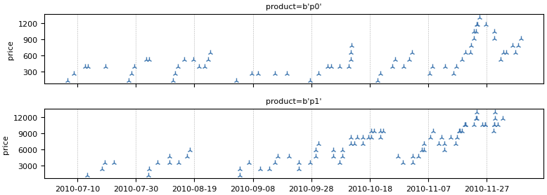
In the previous step, we computed the overall moving sum of sales for the entire shop. However, what if we wanted to calculate the rolling sum of sales for each product or client separately?
For this task, we can use an index.
# Index the data by "product"
sales_per_product = sales.add_index("product")

# Compute the moving sum for each product
weekly_sales_per_product = sales_per_product["price"].moving_sum(
        tp.duration.days(7)
)

# Plot the results
weekly_sales_per_product.plot()
|
 |
Our dataset contains individual client transactions. To use this data with a machine learning model, it is often useful to aggregate it into time series, where the data is sampled uniformly over time. For example, we could aggregate the sales weekly, or calculate the total sales in the last week for each day.
However, it is important to note that aggregating transaction data into time series can result in some data loss. For example, the individual transaction timestamps and values would be lost. This is because the aggregated time series would only represent the total sales for each time period.
Let's compute the total sales in the last week for each day for each product individually.
# The data is sampled daily
daily_sampling = sales_per_product.tick(tp.duration.days(1))

weekly_sales_daily = sales_per_product["price"].moving_sum(
    tp.duration.days(7),
    sampling=daily_sampling,  # The new bit
)

weekly_sales_daily.plot()
|
 |
After the data preparation stage is finished, the data can be exported to a Pandas DataFrame as a final step.
tp.to_pandas(weekly_sales_daily)
|

A key application of Temporian is to clean data and perform feature engineering for machine learning models. It is well suited for forecasting, anomaly detection, fraud detection, and other tasks where data comes continuously.
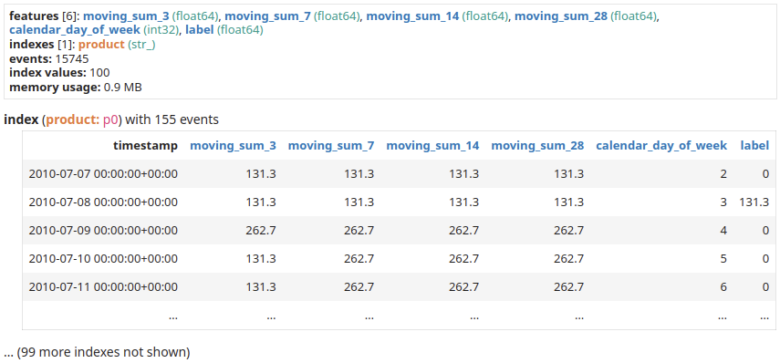
In this example, we show how to train a TensorFlow model to predict the next day's sales using past sales for each product individually. We will feed the model various levels of aggregations of sales as well as calendar information.
Let's first augment our dataset and convert it to a dataset compatible with a tabular ML model.
sales_per_product = sales.add_index("product")

# Create one example per day
daily_sampling = sales_per_product.tick(tp.duration.days(1))

# Compute moving sums with various window length.
# Machine learning models are able to select the ones that matter.
features = []
for w in [3, 7, 14, 28]:
    features.append(sales_per_product["price"]
        .moving_sum(
            tp.duration.days(w),
            sampling=daily_sampling)
        .rename(f"moving_sum_{w}"))

# Calendar information such as the day of the week are
# very informative of human activities.
features.append(daily_sampling.calendar_day_of_week())

# The label is the daly sales shifted / leaked one days in the future.
label = (sales_per_product["price"]
    .leak(tp.duration.days(1))
    .moving_sum(
        tp.duration.days(1),
        sampling=daily_sampling,
        )
    .rename("label"))

# Collect the features and labels together.
dataset = tp.glue(*features, label)

dataset
|
 |
We can then convert the dataset from EventSet to TensorFlow Dataset format, and train a Random Forest.
import tensorflow_decision_forests as tfdf

def extract_label(example):
    example.pop("timestamp") # Don't use use the timestamps as feature
    label = example.pop("label")
    return example, label

tf_dataset = tp.to_tensorflow_dataset(dataset).map(extract_label).batch(100)

model = tfdf.keras.RandomForestModel(task=tfdf.keras.Task.REGRESSION,verbose=2)
model.fit(tf_dataset)
|
And that’s it, we have a model trained to forecast sales. We now can look at the variable importance of the model to understand what features matter the most.
model.summary()
|
In the summary, we can find the INV_MEAN_MIN_DEPTH variable importance:
Type: "RANDOM_FOREST"
Task: REGRESSION
...
Variable Importance: INV_MEAN_MIN_DEPTH:
    1.        "moving_sum_28"  0.342231 ################
    2.              "product"  0.294546 ############
    3. "calendar_day_of_week"  0.254641 ##########
    4.        "moving_sum_14"  0.197038 ######
    5.         "moving_sum_7"  0.124693 #
    6.         "moving_sum_3"  0.098542
|
We see that moving_sum_28 is the feature with the highest importance (0.342231). This indicates that the sum of sales in the last 28 days is very important to the model. To further improve our model, we should probably add more temporal aggregation features. The product feature also matters a lot.
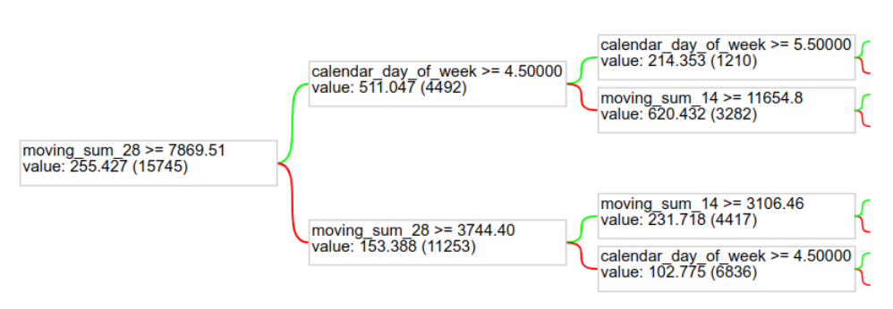
And to get an idea of the model itself, we can plot one of the trees of the Random Forest.
tfdf.model_plotter.plot_model_in_colab(model, tree_idx=0, max_depth=2)
|
 |
We demonstrated some simple data preprocessing. If you want to see other examples of temporal data preprocessing on different data domains, check the Temporian tutorials. Notably:
- Heart rate analysis ❤️ detects individual heartbeats and derives heart rate related features on raw ECG signals from Physionet.
- M5 Competition 🛒 predicts retail sales in the M5 Makridakis Forecasting competition.
- Loan outcomes prediction 🏦 prepares relational SQL data to predict outcomes for finished loans.
- Detecting payment card fraud 💳 detects fraudulent payment card transactions in real time.
- Supervised and unsupervised anomaly detection 🔎 perform data analysis and feature engineering to detect anomalies in a group of server’s resource usage metrics.
We demonstrated how to handle temporal data such as transactions in TensorFlow using the Temporian library. Now you can try it too!
- Join our Discord server, to share your feedback or ask for help.
- Read the 3 minutes to Temporian guide for a quick introduction.
- Check the User guide.
- Visit the GitHub repository.
To learn more about model training with TensorFlow Decision Forests:
- Visit the official website.
- Follow the beginner notebook.
- Check the various guides and tutorials.
- Check the TensorFlow Forum.


september 11, 2023 — Posted by Google: Mathieu Guillame-Bert, Richard Stotz, Robert Crowe, Luiz GUStavo Martins (Gus), Ashley Oldacre, Kris Tonthat, Glenn Cameron, and Tryolabs: Ian Spektor, Braulio Rios, Guillermo Etchebarne, Diego Marvid, Lucas Micol, Gonzalo Marín, Alan Descoins, Agustina Pizarro, Lucía Aguilar, Martin Alcala RubiTemporal data is omnipresent in applied machine learning applications. Data often cha…


