https://blog.tensorflow.org/2019/06/modeling-unknown-unknowns-with-tensorflow-probability.html?hl=bn
https://blogger.googleusercontent.com/img/b/R29vZ2xl/AVvXsEiwYA70Ug9rL2wh6hcVD3NwR91Ik4AXeX9sQbA6GpxRdgcBL3Vr1idHeftWmhAjKOvg8YJhE61ZMzRnVwfXK4Kf8WbbG3z7nFxw2aAHooHkyhyphenhyphenuPwmUS1ucjFqUBgE61ciy7WgPcSQht4A/s1600/fig1.png
Modeling “Unknown Unknowns” with TensorFlow Probability — Industrial AI, Part 3
Posted by Venkatesh Rajagopalan, Director Data Science & Analytics; Mahadevan Balasubramaniam, Principal Data Scientist; and Arun Subramaniyan, VP Data Science & Analytics at BHGE Digital
We believe in a slightly modified version of George Box’s famous comment: “All models are wrong, some are useful”
for a short period of time. Irrespective of how sophisticated a model is, it needs to be updated periodically to accurately represent the underlying system. In the
first and
second parts of this blog series, we introduced our philosophy of building hybrid probabilistic models infused with physics to predict complex nonlinear phenomena with sparse datasets. In particular, in the second installment, we described how to update probabilistic models with newly available information. We were able to model the known unknown behavior of how our physical system would degrade over time by using data from a different, but similar physical asset at a more advanced stage of degradation.
In this final part, we will describe the uncertainties that are characterized as “unknown unknowns” and the techniques used for effectively modeling them. To bring all the aspects of our modeling philosophy together in one application, we will predict the performance of a lithium ion battery when we don’t know its real deterioration characteristics.
Battery Health Model
Battery storage has become critical for various applications, ranging from consumer devices to electric vehicles. Lithium ion batteries, in particular, are widely used because of their high power and energy densities. Modeling the battery performance is very crucial to predict its state of charge (SoC) and state of health (SoH). As a battery ages, its performance deteriorates in a non-linear manner. Significant research has been undertaken to understand the phenomenon of battery degradation and to develop models for predicting battery life. For more details on the causes of battery degradation and the associated modeling, please refer to the rich literature[1].
Cell potential (voltage) and capacity (usually stated in Ampere-hours) are two primary metrics of interest in a lithium-ion battery. The chart below depicts the time-profile of cell potential in a discharge cycle as a function of current draw. As the discharge current increases, the cell potential decreases more rapidly over time.
 |
| Cell potential versus time for different current draws. |
The typical degradation in cell potential, across charge-discharge cycles, for a single current discharge (2.5 A), is shown below. With cycling (i.e., usage), the capability of the battery to deliver a voltage will decrease even for the same current draw. Experimental results validating such behavior can be found here[2,3].
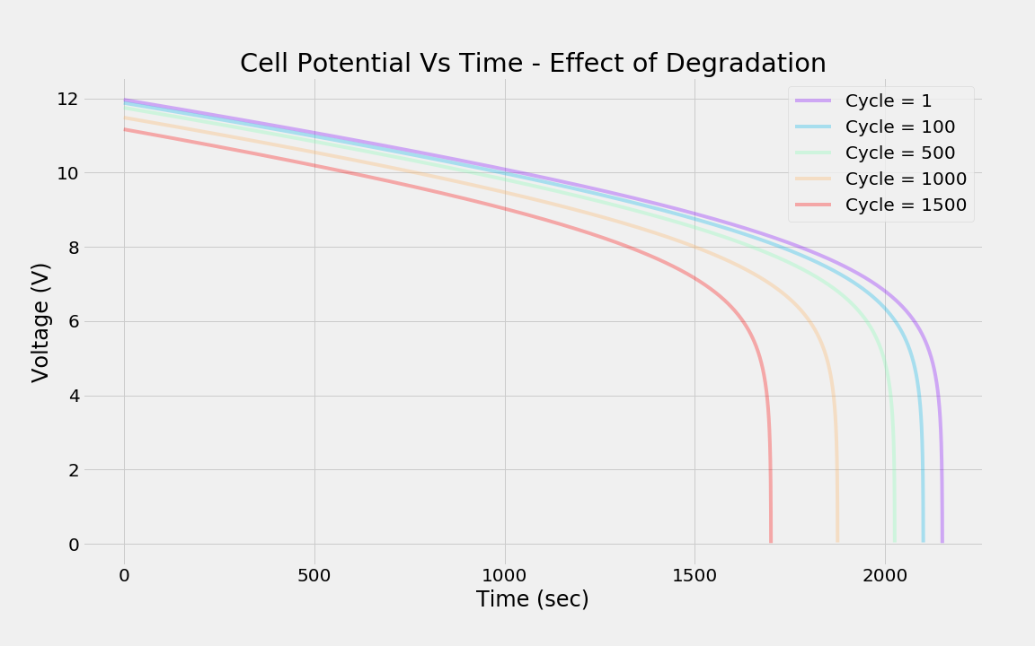 |
| Effect of cycling (usage) on cell potential. |
While there are several approaches for modeling battery characteristics, including physics and hybrid models, we intend to illustrate a data-driven approach for estimating the state of health (or degradation) of the battery when the physics of degradation is unknown. The key advantage of this approach is that the model requires data only from pristine (little or no degradation) batteries and the extent of degradation can simply be tracked as an anomaly (i.e., a change from the nominal behavior) for incipient detection. Further, the model lends itself to continuous updating with measurements — critical for accurate prediction of cell potential. This continuous model updating is required since every customer operation of an asset is unique. We refer to this updating as a
model of one, where we can continuously update the model to track a particular customer’s usage in the field. The challenge is to do this updating in a computationally efficient manner with sporadic, noisy field measurements.
Data Generation
We will use the following equations to generate the discharge curve:
V= a-0.0005*Q + log(b-Q) where a=4–0.25*I and b=6000–250*I
Where
a is the linear decrease and
b is the asymptotic decrease regions as shown in the discharge curves.
I is the discharge current and
Q represents the charge expended by the battery with

The values of
a and
b are notional and representative of discharge curve profiles[4].
Every application is unique and utilizes the battery differently. Consider two dimensions of variation: the amount of discharge and the rate of discharge. Then consider that both of these dimensions can also be applied to the recharging cycle. In other words, a battery can be discharged and recharged fully or partially; it can also be discharged and recharged slowly or quickly. The usage of each battery and variation in manufacturing process affect how each battery degrades. We simulate this variation by choosing a random value for the deterioration parameter δ and computing a response for a random usage at a random cycle. After multiple discharge-recharge cycles, a battery will degrade in performance and provide a lower voltage and lower overall capacity. To illustrate the concept of degradation tracking with a simple example, we will model the deterioration by functionally altering the linear and asymptotic segments of the battery for the entire cycle by a deterioration factor.
If δ is the deterioration factor, then modified battery responses would be the following:

The data from degraded batteries are used for model updating, and not for building the initial model. Please note that this functional form is only an approximation but still representative of field behavior of a battery.
Known Unknowns versus Unknown Unknowns: With the above dataset, this problem can be cast either as a known-unknown case or an unknown-unknown case. This problem can be solved as a known unknown case, if the modeler knows the physics equation that describes the degradation phenomena and thus understands the specific way in which the degradation parameter (δ) interacts with the physics equation. Knowing these specific details, the modeler can cast this as a model update problem as described in the
second part of our blog series.
However, if the underlying physics is unknown, then the modeler has no option but to use the
“raw” data from pristine batteries to build a data-driven model and then update the data-driven model as the model performance deteriorates. Without specifically knowing the degradation mechanism, the modeler may be left with no choice but to update a large section of the data-driven model. The hope is that there are sufficient degrees of freedom in the model and sufficient information in the new dataset to update the model accurately. In real-world applications of solving for unknown unknowns, it is common for these conditions to occur.
We will show the latter case of modeling the unknown unknown here by building a DNN model with the data from pristine batteries. We have provided representative values to ensure the reader can create the data to build a “generic” deep learning model.
The process that we will follow for the rest of the blog is shown below:
 |
| Modeling process to illustrate unknown unknowns. |
The simple DNN model architecture shown below with 5 hidden layers (4,16, 64,16,4) will be used for illustrating the concepts.
 |
| Simple Deep Neural Network architecture to model battery performance. |
Training the DNN with up to 200 epochs produces a sufficiently accurate model as shown below. Both training and test points are reasonably predicted for the pristine battery.
 |
| Training and test predictions from DNN model. |
We will add a non-linear degradation to the pristine battery as described above. The specific instance of the degraded battery performance is shown by the blue dots below for a degradation parameter (δ) of 0.163. Based on actual usage, the blue dots denote actual measurements of a battery during a discharge cycle.
 |
| Pristine DNN model predictions compared to degraded battery data. |
Adding degradation almost immediately makes this model inaccurate. Since we don’t know the exact mechanism of degradation, we will choose to update the hyperparameters of the last hidden layer[5], with a particle filter.
Model Updating with Particle Filter
Particle filtering (PF) is a technique for implementing a recursive Bayesian filter by Monte Carlo simulations. The key idea is to represent the posterior density function with a set of random samples with associated weights; we compute estimates based on these samples and weights. As the number of samples becomes very large, the PF estimate approaches the optimal Bayesian estimate. For an extensive discussion on the various PF algorithms, please refer to this
tutorial.
As with the Unscented Kalman Filter (UKF) methodology described in our previous
blog post, we will model the “states” of the PF as a random walk process. The output model is the DNN. The equations describing the process and measurement models are summarized below:
x[k] = x[k-1] + w[k]
y[k] = h(x[k], u[k]) + v[k]
where:
- x represents the states of the PF (i.e., the hyper-parameters of the DNN that need to be updated)
- h is the functional form of the DNN
- u represent the inputs of the DNN: current and capacity
- y is the output of the DNN: cell potential
- w represents the process noise
- v represents the measurement noise
The PF algorithm makes no assumptions other than the independence of noise samples in the process and measurement models.
The particle filter is robust for updating the DNN model with field measurements as well as versatile enough to be used for model training. Refer to this
paper for a detailed discussion. The salient steps of the PF-based model update methodology are summarized below:
- Generate initial particles from a proposed density, called the importance density
- Assign weights to the particles and normalize the weights
- Add process noise to each particle
- Generate output predictions for all the particles
- Calculate likelihood of error between actual and predicted output value, for each particle
- Update a particle weight using its error likelihood
- Normalize the weights
- Calculate effective number of samples
- If effective number of samples < Threshold, then resample the particles
- Estimate the state vector and its covariance
- Repeat steps 3 to 10, for each measurement.
The PF-based methodology for updating the DNN model has been implemented as a
Depend On Docker project and can be found in this
repository, and in this Google
Colab. As stated earlier, PF assumes only that the noise in the process and measurement model are independent. Accordingly, we need not assume that the noise follows a Gaussian distribution, in contrast to the UKF assumptions. Thus, the extensive functionality provided by TensorFlow Probability’s
tfp.distributions module can be used for implementing all the key steps in the particle filter, including:
- generating the particles,
- generating the noise values, and
- computing the likelihood of the observation, given the state.
Code snippets for a few steps of the algorithm are provided below.
Generating initial set of particles
The particle filter is initialized with a set of particles generated using TF Probability.
import tensorflow as tf
import tensorflow_probability as tfp
tfd = tfp.distributions

# Generate Particles with initial state vector pf['state'] and state covariance matrix pf['state_cov']
sess = tf.Session()
state = np.array(pf['state'])
state.shape = (num_st, )                                  # num_st is the number of state variables
mvn = tfd.MultivariateNormalFullCovariance(loc=state, covariance_matrix=pf['state_cov'])
particles = sess.run(mvn.sample(pf['Ns']))                # pf['Ns'] is the number of particles to be generated
Generating output for each particle
Output predictions are generated for every particle by setting the particle values to the bias and the weights of the last layer of the DNN and running the model.
def pf_predout(coef, loc_pm, p_ampDraw, time_val, tVarDict):

    p_ampSec = p_ampDraw * time_val
    baseW_Out = tVarDict['W_OUT:0']
    n_dim = len(coef)

    coef = np.array(coef)
    coef.shape = (n_dim,)

    tVarDict['b_OUT:0'] = [coef[0]]
    for idxW in np.arange(len(baseW_Out)):
        baseW_Out[idxW, 0] = coef[idxW + 1]
    tVarDict['W_OUT:0'] = baseW_Out

    yhat = np.asmatrix(loc_pm.predictSingleRowAugmented(p_ampDraw, p_ampSec, tVarDict))

    return yhat
Updating weight of each particle
Once the predictions have been generated, the likelihood of a particle being in the true state is calculated and the weight associated with that particle is updated accordingly.
def update_weights(y, yhat, R, prev_weight):
    from scipy.stats import norm

    likelihood = norm.pdf(y-yhat, 0, R)
    updt_weight = prev_weight * likelihood

    return updt_weight
Resampling the particles
Particles are resampled, if required, through systematic resampling.
def systematic_resample(sess, weights):
    N = len(weights)

    # make N subdivisions and choose positions with a random offset
    positions = (sess.run(tf.random.uniform((1, ))) + np.arange(N)) / N

    indexes = np.zeros(N, 'i')
    cum_sum = np.cumsum(weights)
    i, j = 0, 0
    while i < N:
        if positions[i] < cum_sum[j]:
            indexes[i] = j
            i = i + 1
        else:
            j = j + 1
    return indexes

  def resample_from_index(particles, weights, indexes):
    particles = particles[:, indexes]
    weights = weights[indexes]
    weights.fill(1.0 / len(weights))

    return particles, weights, indexes
Results and Discussion
Updating the last layer of weights and biases of the baseline DNN model with the first datapoint using the particle filter produces the model predictions shown below in green. The shaded region signifies the prediction uncertainty computed using 500 random particles.
 |
| Updated model prediction (from 1st update point). |
The algorithm chooses the next update point as the time at which the observation falls outside the prediction uncertainty. In this case, it is the time point 13 (close to 700 seconds). Incrementally updating the model whenever the observed data falls beyond the model prediction uncertainty produces the desired accuracy as shown below.
 |
| Sequential model update results initiated based on prediction uncertainty. |
Combining all the models together, we get the prediction across the entire degradation cycle. Clearly the baseline model misses the degradation completely resulting in a 50% error in voltage predictions at the end of the battery cycle. Simple updates with prediction uncertainty thus enables the modeler to account for “unknown unknowns”.
 |
| Final model (only latest updates) predictions compared to initial model. |
 |
| Comparison of model prediction errors. |
For the last hidden layer of four nodes, we depict below the initial state of the battery model and the final updated state. Clearly, the state has changed significantly and the model predictions improve even though the updates were performed with only a few data points. The change in the state distributions can also be viewed as an indication of the anomaly (in this case, the deterioration δ) in the system. Thus, these plots indicate that there was sufficient information in the data to update the models. By contrast, updating the model with data sets that do not have any relevant information will result in the model continuing to be inaccurate. Thus, choosing the right time to update the model is as important — or more important — as the method used to update the model.
 |
| Comparison of initial and final state of the parameters of the last DNN hidden layer. |
Summary
Making AI real in the industrial world requires a combination of several disciplines: domain knowledge, probabilistic methods, traditional machine learning, and deep learning. We have shown the techniques to combine effectively these disciplines to model real-world phenomena with limited and uncertain data. The third part of this series of blogs focused on modeling “unknown unknowns”. To build a digital twin of an industrial asset, it is essential to build a model of “one” — where the model continuously adapts to track field measurements over time for every single “asset” in the ecosystem. The particle filter methodology for updating the weights and biases of a DNN layer built on pristine data, can be used to build the model of “one”.

In real-world industrial applications, there are many challenges that limit the quantity of useful data, including noise, missing values, and inconsistent measurements. Therefore, choosing what to model, selecting an appropriate modeling methodology (physics, data-driven or hybrid), and choosing which parameters to update continuously are critical to maintaining useful models.
Acknowledgments
This blog is a result of the hard work and deep collaboration of several teams at Google and BHGE. We are particularly grateful to Mike Shwe, Josh Dillon, Scott Fitzharris, Alex Walker, Fabio Nonato and Gautam Subbarao for their many edits, results, code snippets, and — most importantly — enthusiastic support.


